|
|||||||
|
||||||||
This simple tutorial describes the steps that you might go through when using LandSerf for terrain analysis. You can follow the steps using the sample data provided with LandSerf or you can adapt it to use with your own Digital Elevation Model.
Start LandSerf either by selecting it from the Start menu (Windows)
or by typing LandSerf from the command line (UNIX).
The first stage of any terrain analysis is to import a digital model of the land surface to analyse. Most of LandSerf's functionality concerns processing Digital Elevation Models (DEMs). A DEM is simply a matrix of elevation values that describes the height of some surface at regular spatial intervals.
For this tutorial, we shall import a DEM representing part of Columbia River area in Washington, USA.
You may wish to substitute an alternative area of interest (in which case you may wish to look at
details on importing elevation models). The DEM we wish to
import for this exercise is in the ArcGIS ASCII raster format (the text format for rasters used
by the software ArcGIS) and is located in the data sub-directory of the LandSerf
installation. To import this file:
File->Import->ArcGIS Raster Text File... menu.Lincoln.grd from the
data directory.LandSerf will now read the selected file and store it in memory. As we shall perform some alterations to the DEM, we need to save a copy of the file:
File->Save Raster... menu item and save
it as Lincoln.srfdata directory.
This will save the DEM in LandSerf's own format for later retrieval.
If you haven't just moved on from the previous step, you will need to load the DEM into LandSerf:
File->Open Raster... menu item and choose the file Lincoln.srf.
To display this DEM in LandSerf:
Display->Raster menu item. |
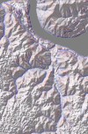
This should display a white rectangle with a faint purple outline of a river channel and a dark green border. The border cells are classified as being 'no data' and result from the Universal Transverse Mercator (UTM) projection used. This USGS DEM file indicates 'no data' cells by coding them as -32766. |
We can confirm this by examining the raster information:
Info.->Raster Information menu
item which should display details of the Lincoln DEM. |
Notice that the range of elevation values is shown as -32766.0 to 887.0. Click
the OK button when you have finished looking at the raster
information.
|
We shall improve the quality of the displayed image by reclassifying the border cells from -32766 to 0. We can do this by 'flooding' the DEM so that no elevation values are less than 0m above sea level:
 |
|
We now have a DEM which ranges from 0 - 887m height (you can confirm this by displaying the Raster Information again). We will now rescale the colours associated with each raster so that it reflects the new distribution:
 |
|
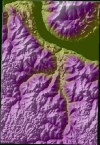 |
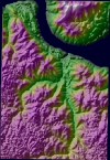
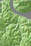
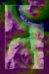
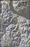
After a few seconds you should now see a full colour image of the DEM. We can
improve the image further by showing the shaded relief of the area (that is,
introducing localised shadow effects on the surface):
|
We shall save a copy of these modifications by resaving the DEM:
File->Save Raster... menu item and save
it as Lincoln.srf
If you haven't just moved on from the previous step, you will need to load the DEM into LandSerf and display it:
File->Open Raster... menu item and
choose the file Lincoln.srf.Display->Relief menu item to display a shadowed
surface representation of the DEM.
To be useful, a DEM file consists of more than a collection of elevation values. The file should also contain information on where the DEM is located, where the boundaries of the region are, and how large each grid cell is. We may also store optional information such as the colour to associate with each elevation value, and a textual description of the region. Such information is collectively known as metadata.
We have already associated some metadata with the DEM, but in this section we shall further modify the colours associated with the DEM and add a more useful textual description.
The first thing we might choose to do is to colour the large river (the Columbia) blue. To do this we need to know its height so that we can associate all cells at that height with the colour blue. To find the height of the river, we can interrogate the DEM interactively:
 |
|
Because the river is the lowest point in the DEM, we can take this opportunity to 'flood' the border cells to this height as we did in Step 2:
Transform->Transform Raster Values... menu
item. Click the Flood checkbox item, and this time enter the
height of the river (393.0) in the 'flood' text field before pressing OK.You should notice that the border cells are now the same murky green colour as the river. Once again, we shall edit the colours to reflect the new range of elevation values:
Edit->Edit Raster Colours menu
item to bring up the colour editor. Click the Default Colours
button to rescale the colours to the new range.Before leaving the colour editor we shall add a new colour rule that tells LandSerf to colour the river a dark blue. To do this, you need to know a little about how colour rules are defined in LandSerf.
Rather than explicitly identify a colour for each height in a DEM, LandSerf allows colour rules to be defined which specify a range of colours to be associated with a range of elevation values. A colour rule consists of two colours and two elevation values. The first colour is associated with the lower of the two elevations, the second colour is associated with the higher elevation. If any DEM cells fall between the two elevations declared in the rule, LandSerf will interpolate colours. Thus if we were to associate the lowest elevation in a DEM with a deep red colour, and the highest with white, our DEM would appear in shades of pink.
Colours are specified as sets of four numbers R,G,B,A that represent red, green, blue and alpha (transparency) components of the colour respectively. Each of these values range between 0 (absence of that component) to 255 (maximum of that component).
If you look at the colour rules shown in the colour editor, you should see that the first rule is 393.0: 0,50,0,255 --> 516.5: 0,150,0,255, meaning that elevation values of 393.0 are coloured dark green, elevations of 516.5 are coloured lighter green and any values between these values will be coloured an appropriate shade of green.
So we are now in a position to alter the colour rules to make the river Columbia dark blue:
 |
After a few seconds pause, the shaded DEM should now appear with a dark blue river. |
The other metadata we shall change in this section will be the title, boundary and notes associated with the raster:
 |
|
Before leaving the raster editing dialogue, we will 'zoom in' slightly so that we lose the dark blue
border cells that surround the DEM. The easiest way to do this is to adjust the values in the
North:, South:, East:
and West fields of the dialogue.
North:, South:, East:
and West values are updated automatically as you do this. When you are
happy with the chosen area, click the Extract Subset of Raster checkbox
and click OK.You should now find that the DEM displayed in the main window now no longer has any blue border cells. It should now also have a more useful set of metadata associated with it. We will save a copy of the DEM before moving on to the next stage:
File->Save Raster... menu item and save it as
Lincoln.srf
If you haven't just moved on from the previous step, you will need to load the DEM into LandSerf and display it:
File->Open Raster... menu item and
choose the file Lincoln.srf.Display->Relief menu item to see a visual representation
of the DEM.We have already gained some impression of the landscape represented by our DEM simply by visualising it. We can assume for example that the landscape contains a large meandering river, some apparently mountainous region to the north, several tributaries flowing from the south of the DEM northwards into the river. We might characterise the region as a whole as 'hilly'.
Such description however has obvious limitations. It is subjective (you may have gained a different impression of the same landscape), it is rather vague (what exactly does 'hilly' mean?), and might simply be incorrect (are we sure that is a mountain to the north of the river or is it just a small undulation?). We can use LandSerf to provide us with a more systematic and objective description of the landscape; one that we can use to compare with other landscapes described by other people.
Firstly it is useful to make sure we have a good idea of the scale and extent of the landscape. We can do this by viewing the metadata associated with the DEM:
Info->Raster Information menu item and look at the
information shown. |
The window includes information on the number of rows (about 450 or so depending on how you subset the DEM in the previous step) and columns (about 300 or so) in the DEM as well as the size of each grid cell (30m x 30m). This means that we are viewing a landscape that is approximately 10km east-west by 14km north-south. We also know that the range of heights within this regions is 393m to 887m - a vertical range of about 500m. This vertical range or relief only gives us a broad summary of how elevation changes over the surface. |
We can get a more detailed view by visualising the frequency distribution of heights over the surface:
OK
button and select the Info->Raster Histogram menu item. |
We are now presented with a graph of the frequency of height values at 1m intervals. You should
notice that by far the most frequently occurring elevation value is 393m, which corresponds to the
height of the river Columbia. You can calculate the histogram to ignore values at this elevation
by clicking the |
Category width slider to increase the
number of DEM cells that fall in each class. Hold the mouse button down over this arrow until the width
is about 40m.The modal (most frequent) category now corresponds to the (purple) plateau area in the south-west of the region. Note that the shaded relief image of the same region suggests a quite 'rough' terrain here, even though most of the variation in height is within about 10m.
So can we get a better idea of the 'roughness' of the terrain? One way of doing this is to measure the steepest slope at all cells in the DEM and visualise the results:
Analyse->Calculate Surface
	Parameter
menu item. Select Slope from the list of properties
and press the OK button.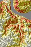 |
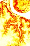
You should see a message Calculating Surface Parameterisation appear at the bottom of the LandSerf window and a percentage progress indicated in the bottom left corner. After 10 seconds or so, a new slope image should be displayed. Slope is coloured from white (horizontal) through yellow to red (steepest slope). This new image shows the flat plateau in the south-west and the steeper slopes bordering the Columbia and its larger tributaries. |
By calculating slope of the DEM, LandSerf has actually created a second raster layer. The first contains the elevation values (the surface), the second the steepest slope at each cell in the DEM (the drape). The shaded relief map that you are currently viewing uses the surface to calculate the shadowing effect, and the drape to create the white-yellow-red component. You can view the slope map by itself by selecting the drape:
 |
|
We can analyse this raster in much the same way as we did for the DEM:
 |
|
We shall save a copy of this slope surface for later analysis:
File->Save Raster...
menu item and save it as LincolnSlope.srfSlope represents one of the four surface parameters that are often used to characterise surface behaviour. The other three are aspect which identifies the azimuthal direction of steepest slope, profile curvature, which describes the rate of change of slope in profile, and plan curvature, which describes the rate of change of aspect in plan. We shall use LandSerf to view each of these in turn:
Edit->Set Processing to > Surface menu item. After a few seconds pause,
the shaded relief map with slope should be redisplayed.Analyse->Calculate Surface Parameter
menu item, choose Aspect from the list of properties
and press the OK button.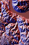 |
 |
 |
Finally, we shall examine one further characterisation of the surface. Rather than measure surface parameters we can classify the terrain into surface features using some of the parameters we have already investigated. One of the commonest (and most useful) classifications is to group all points on a terrain into one of the following:
This can be done by measuring both the slope and curvature of each cell in the DEM and performing the appropriate classification (for more details on how this may be done see the technical details on surface characterisation). We shall perform such a classification on our DEM:
Edit->Set Processing to > Surface), select the
Analyse->Calculate Surface Parameter menu item, and choose the
Feature Extraction item.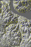 |
After a few seconds, you should see a predominantly grey, blue and yellow image appear. The grey areas represent planar regions, blue areas represent channels and yellow ridges. If you look carefully (you may have to enlarge the LandSerf window), you should also see occasional red cells that represent local peaks in the landscape and green cells that represent passes in the landscape. |
Feature classifications like this are useful for several reasons. The pattern of channels appears somewhat similar to a drainage network, thus giving us an idea of where water would flow over the surface. Perhaps less obviously the pattern of yellow cells gives us an equivalent ridge network, identifying portions of the landscape where water is likely to flow from. Consequently, the ridge network is related to the drainage divides/watersheds that define drainage basins. In theory at least, the green passes identify points of intersection between the channel and ridge networks. Along with pits and peaks, passes represent what are sometimes called surface specific points - points on the landscape that carry special significance in its structure.
Before leaving this section you should save a copy of these surface features for later analysis:
Edit->Set Processing to > Drape), select the File->Save Raster...
menu item and save it as LincolnFeatures.srf
Before continuing with this section, make sure you have the Lincoln DEM loaded and the processing set to the surface:
Edit->Set Processing to > Surface.
File->Open Raster... menu item and
choose the file Lincoln.srf.Display->Relief menu item.When we wish to characterise a real terrain using a computer, the closest we can get is to characterise the elevation model that represents it. In doing so we hope that the model is sufficiently accurate for the purposes of analysis. As far as possible we should strive to produce characterisations of landscape that are independent of the particular model we have used.
One of the most significant limitations of the models and processing we have carried out so far has been the scale of analysis implied by the DEM resolution. You will remember that each cell in the Lincoln DEM is 30m x 30m. Since most of the analytical functions we have used so far work by comparing one cell with its 8 adjacent neighbours, the results of that analysis are likely to be at the resolution of approximately 3 times the grid cell size. So for example, the blue valleys we identified in the previous section will be those that have a width of about 30-90m. This scale is really rather arbitrary; we might be more interested in characterisation of features have expression over 1km or 10 cm. Unfortunately, the DEM cannot provide us with direct information at a finer scale than its resolution (30m), but we can use it to perform analysis at a broader scale.
The basis for most of the analytical functions in LandSerf is the process of quadratic approximation (see details on surface characterisation for further information). This involves taking a local window of DEM cells (3 x 3 in the examples we have seen so far), and fitting the most appropriate continuous quadratic function through them. LandSerf then uses this quadratic function to calculate parameters such as slope and curvature. We can set the size of the local window that LandSerf uses before it does any calculation. This allows us to perform analysis at much broader scales than that implied by the DEM resolution.
As a first step, we will view the effect of changing window size by smoothing out features that are smaller than about 350m wide. Since each cell is 30m, we will need to process the surface using window sizes of 11x11 cells rather than 3x3:
Configure->Set Window Scale... menu item and set the
window size to 11 rather than 3 (we shall leave the 'distance decay exponent' set to 0). Press
the OK button close the dialogue box.By changing window scale, any subsequent analysis will be performed at this new 350m scale. To demonstrate this effect we shall reinterpolate our DEM at the new scale:
Analyse->Calculate Surface Parameter menu item, and choose
the Elevation item. You will notice that processing at this new scale
takes longer than previous examples since LandSerf is having to process 13 times as many cells
for each calculation.
Edit->Set Processing to > Drape).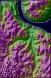 |
The result of broadening the scale of analysis is to smooth out many of the finest scale details while leaving the larger features of the landscape unaltered. You should also notice a border around the entire raster. This is produced because analysis based on square windows of size n x n cannot process cells within (n-1)/2 cells of the edge. |
We can see the effect of further broadening the scale of analysis by setting the window size to 65:
 |
|
So do the parameters that we can measure from the surface also vary if we calculate them at this new broader scale? We can find out the answer to this question by measuring a surface parameter at many different scales and seeing how it varies:
Edit->Set Processing to > Surface)
and select the Info->Multi-scale query... item. Choose
aspect and click on various points on the DEM. |
You should be presented with a new window that displays concentric circles in the top half (you may have to resize the window if the circles appear elliptical), and sets of four numbers in the bottom half. The graphical display shows how aspect varies with scale. The line drawn on the graph shows the direction of steepest slope measured from 3 x 3 windows at the centre to 65 x 65 cell windows at the outer edge. If the line remains in a relatively constant direction, aspect is said to be scale-invariant at this location. If the line appears to meander as it moves out from the centre, the slope direction must be dependent on the scale at which it is measured. A numerical measure of this dependency is shown in the bottom half of the window. The first two numbers give the location of the point being queried, while the second two give the (circular) mean and standard deviation of the aspect measure. |
If you try dragging the mouse over the DEM, the aspect graph is updated continuously. This allows you to investigate the spatial pattern of scale dependency. Which parts of the landscape produce scale-invariant measures, and which produce scale-dependent measures?
Try examining the scale dependency of other measures:
Info->Multi-scale query... item.
Choose Profile curvature and click on various points on the DEM. Try to
relate the curve plotted and the location and character of the landscape you have
queried. If you hold the mouse button down over any location on the landscape, a white square will appear
giving a graphical indication of the maximum window size.One of the advantages of multi-scale processing of terrain, is that we can relate our analysis to scales that are of most interest to us. We shall round of this section by calculating the network of surface features at two different scales. First we shall identify the network of ridges and channels at a fine scale:
Configure->Set Window Scale... menu item and set the
window size to 5 and the distance decay exponent to 1.0. Press the OK
button to close the dialogue box.This has set the processing back to using a 5 x 5 cell window, but additionally, by specifying a positive distance decay value, we have told LandSerf to give a greater weighting to cells nearer the centre of a window, than ones that are further away. The higher the value of this exponent, the greater the importance given to near cells.
 |
|
We can improve the representation of the network by forcing LandSerf to connect some of these ridges and channels together. As this network would describe the topology of the surface, LandSerf will represent it using a vector rather than raster coverage:
 |
|
Notice how both the blue channel network and the yellow ridge network appear similarly tree-like. The plateau to the south-west is dominated by local passes, pits and peaks (green, black and red dots). This is because at this scale, errors in the DEM tend to dominate flatter regions. We can broaden our scale of analysis, and therefore reduce the impact of DEM error, by repeating the process using a larger window size:
 |
|
Notice how that at this broader scale, the plateaux areas are largely free of ridges and channels. The area to the north or the meander consists of a crescent shaped drainage divide and a simple network draining out to the east.
You may wish to save a copy of this vector network for later analysis:
File->Save Vector...
menu item and save it as Network15.vecThis ends the tutorial. This has been an introduction to LandSerf and the process of terrain analysis. To get the most of the package, you will have to experiment with some of the other functions available and apply them to your own DEMs. See the user guide for more details.
