Tutorial: Images as Two-Dimensional Signals in Matlab
Contents
Images as a 2D matrices
The simplest way of thinking of an image as a grid of points, or elements and each of them will contain a certain value. The value of the element is related to the colour or intensity of the image itself. In the technical jargon, the grid is called a "matrix" and each point of the grid is called a "pixel" which is the combination of the words "picture element". The images we will refer to along this text will all be digital images and the size of the grid will define the resolution of the image. When data sets contain volumetric information, like those acquired from Magnetic Resonance Images or multiphoton microscopes, the elements are related to a volume and thus the "volume elements" are called "voxels". There is no specific term to describe the elements of data sets with higher dimensions.
The size of an image varies widely, for example, it may be a square of 128 x 128, 256 x 256 or 512 x 512 pixels or it may depend on the resolution of the cameras used to capture the image. In the general case an image can be of size m-by-n, 'm' pixels in the rows or vertical direction and 'n' pixels in the columns or horizontal direction. The value or intensity of the pixels can be related to light intensity, attenuation, depth information, concentration of a fluorophore, or intensity of radio wave depending on the type of acquisition process through which the image was captured.
This intensity level of each pixel is the essential information that forms the image. The intensity values of the pixels are also used to perform operations like segmentation or filtering. In addition, we can use the intensity to extract useful information; like number of cells in an image. In other cases, the relationship between the intensities of neighbouring pixels and their relative variation may be of interest, as it is in texture analysis.
The intensity level of a grey scale image describes how bright or dark the pixel at the corresponding position should be displayed. There are several ways in which the intensity of each pixel is recorded. For example, a pixel may have one of two options, 0 or 1, where 0 will be displayed as low intensity (or black in some cases) and 1 will be displayed as high intensity (or white). These two options correspond to what is called in mathematical terms as 'logical' or 'Boolean' data types.
The size of an image varies widely, for example, it may be a square of 128 x 128, 256 x 256 or 512 x 512 pixels or it may depend on the resolution of the cameras used to capture the image. In the general case an image can be of size m-by-n, 'm' pixels in the rows or vertical direction and 'n' pixels in the columns or horizontal direction. The value or intensity of the pixels can be related to light intensity, attenuation, depth information, concentration of a fluorophore, or intensity of radio wave depending on the type of acquisition process through which the image was captured.
The intensity level of a grey scale image describes how bright or dark the pixel at the corresponding position should be displayed. There are several ways in which the intensity of each pixel is recorded. For example, a pixel may have one of two options, 0 or 1, where 0 will be displayed as low intensity (or black in some cases) and 1 will be displayed as high intensity (or white). These two options correspond to what is called in mathematical terms as 'logical' or 'Boolean' data types.
Colour images contain important information about the perceptual phenomenon of colour related to the different wavelengths of visible electromagnetic spectrum. In many cases, the information is divided into three primary components Red, Green and Blue (RGB) or psychological qualities such as hue, saturation and intensity. Prior knowledge of the objects colour can lead to classification of pixels but this is not always known. In Matlab, a two-dimensional matrix is assumed to be a grey-scale image, and a three-dimensional with any number of rows and columns and 3 levels is assumed to be an RGB colour image. We will soon learn that 2D images can be displayed with different "colour maps", which are not related with the RGB components of a colour image.
A useful source of images, which in many cases are released in the public domain, freely licensed media file repository and "may be used, linked, or reproduced without permission" is the Wikipedia (http://www.wikipedia.org/) and the Wikimedia Commons (http://commons.wikimedia.org/wiki/Main_Page).
The command 'imread' is quite powerful as it automatically checks the format in which the image was saved (jpeg, tiff, bitmap, etc.), which may or may not be compressed, and then assigns the values of the pixels into a 2D or 3D Matlab matrix. A very useful quality of 'imread' is that it can also read images that are located anywhere on the Internet (as long as they are not behind firewalls or password-protected). Instead of typing the path to the folder in a local computer, we can use the location of the image on a website like this:
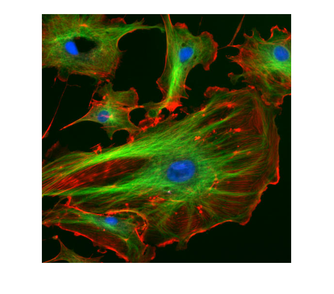
fluorescent_cells = imread('https://upload.wikimedia.org/wikipedia/commons/0/09/FluorescentCells.jpg');
We can see that the image corresponds to a series of cells that have been fluorescently labelled with the colours red, green and blue. (Author Jan R Benutzer, uploaded 4th December 2005).
Displaying images
With the previous line we have read an image and stored it in the variable called 'fluorescent_cells', which we can display with the command 'imshow' like this:
imshow(fluorescent_cells)
Alternatively we can use the command 'imagesc' which scales the images and does not keep the proportions of the axes, we will see more of this later.
Besides the display of an image, we may be interested in knowing its dimensions. We can find out using the command 'size', and we can store the results in three variables, one for each dimension of interest:
[rows,columns,levels] = size(fluorescent_cells)
rows =

   512


columns =

   512


levels =

     3
We can see that the image contains a number of rows and columns and 3 levels or colour channels.
Red blood cells
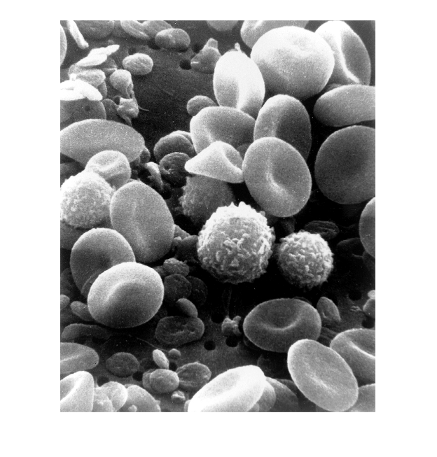
Let's try another image from wikipedia, one image of normal circulating human blood observed with a scanning electron microscope (authors Wetzel and Schaefer, February 1982), like this:
blood_cells = imread('http://upload.wikimedia.org/wikipedia/commons/8/82/SEM_blood_cells.jpg');
In the previous line, we instructed Matlab to read an image (imread) from a website (the Wikimedia Commons address) and store it in a local variable (blood_cells). Before we display the image, we may be interested in knowing its dimensions. We can find out using the command 'size', and we can store the results in three variables, one for each dimension of interest:
[rows,columns,levels] = size(blood_cells)
rows =

        2239


columns =

        1800


levels =

     3
We can see that the image contains 2239 rows, 1800 columns and 3 levels. To display the image we use the command 'imshow'. In order to keep the previous image open, we will display the image in a new window or figure, we can do this by opening the figure before displaying it:
figure
imshow(blood_cells)
The image of the blood cells is a "grey-scale" image, as each pixel contains information related to a level of grey between 0 and 255. Besides grey-scale, we may be interested in black and white images (purely black and white, without any intermediate greys) which are also called binary images, and colour images.
In some cases, it may be the case that the image is too big to fit in the screen and will be scaled down. This is one of the properties of the command 'imshow', which is special for images. We can also use the command 'imagesc' (image-scale), which provides more options for image analysis:
figure
imagesc(blood_cells)
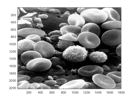
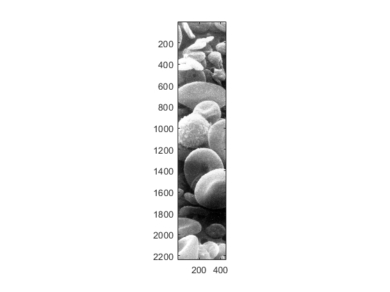
There are some important differences between the commands 'imshow' and 'imagesc'. First, the axes along the rows and columns are normally shown with 'imagesc' whilst with 'imshow' they are hidden. Second, 'imshow' will scale automatically vertical and horizontal dimensions so that the pixels have the same dimensions in rows and columns, at the same time, it scales the size of the window proportionally to the image. On the other hand, 'imagesc' opens a standard size window and will adjust the size of the rows and columns to the size of the window, thus the pixels do not necessarily have the same dimensions in rows and columns. To further illustrate these differences, we can try the following command, which will plot only a quarter of the columns of the blood cells image:
figure
imagesc(blood_cells(:,1:end/4,:))

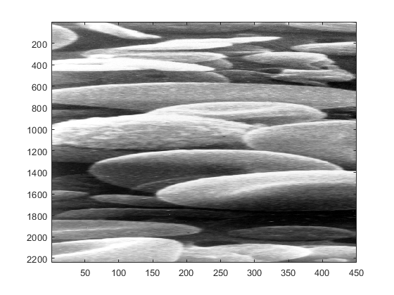
To keep the vertical and horizontal axis in the same proportion we can use the following command:
axis equal
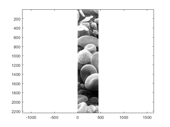
and to remove the white space around the image we can use this command:
axis tight
If we want again to fill the image we simply change the axis with the following command:
axis normal
The windows in the screen can be modified in size by using the mouse and clicking on the edges or corners of the image and changing its dimensions (in some Macs you can only change by clicking on the bottom right corner).
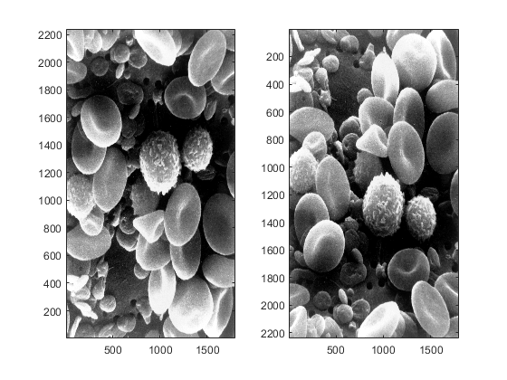
There is another important use of the command 'axis'. In the figures that we have observed so far, the rows and columns begin in the top left corner, and grow downwards and to the right. In contrast, when we display signals, the coordinate system normally starts in the bottom left corner and grows upwards and to the right. In Matlab, the system where the origin (the place where the numbering starts) is at the bottom left is considered the default Cartesian system (or Cartesian axes mode) and is obtained by writing the letters 'xy' after the command 'axis'. The alternative system with the origin at the top is obtained by writing the letters 'ij'; this system is called the "matrix axes mode". We can observe the two systems together in the following figure:
figure
subplot(121)
imagesc(blood_cells)
axis xy
subplot(122)
imagesc(blood_cells)
axis ij
Thresholding and Histograms
Probably the most common single element mapping is to threshold an image. That is, to compare the intensity of each pixel of the image against one level or threshold so that all those above (or below) the threshold are placed in one group, say foreground, and the others into another, like a background. For example we can select two values of intensity and threshold the image with them. Since we have no knowledge of the distribution of intensity levels of the image we can investigate this by obtaining a histogram with the command 'hist'. But before calling the histogram, we need to convert the image into a new data type called "double" as you cannot perform some mathematical functions on the original data type of "uint8".
figure
image1 = double(blood_cells);
hist(image1(:))
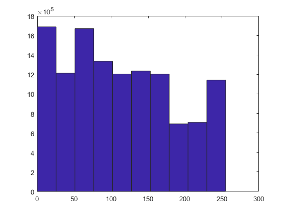
By default, the histogram will be divide the intensity levels into ten groups or "bins" in which the occurrence of the pixels will be counted. Notice that we have re-arranged the image, which has rows, columns and 3 levels, into a single column by using the operator (:). Since 10 bins may not give a good idea of the distribution, we can increase that to a given number, say, 20 or 50, or we can indicate instead of a number of bins, a range. We will do that from the minimum value of the image, to the maximum value like this:
figure
hist(image1(:),[min(image1(:)):max(image1(:))])
axis tight
grid on
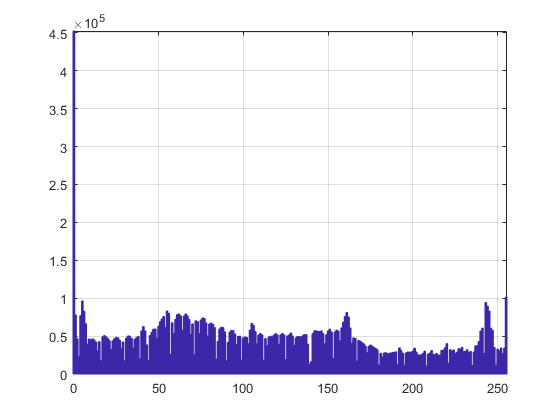
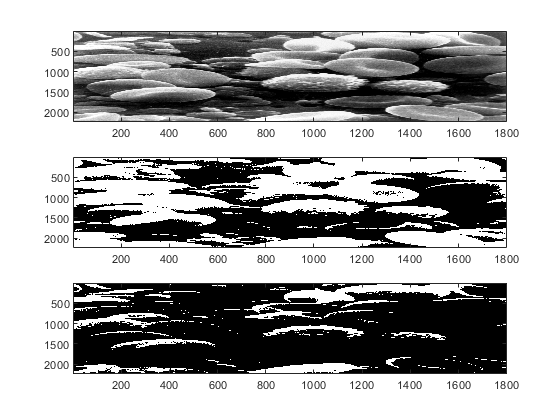
We can now see that this image spreads the intensity levels between 0 and 255, which is common of pictures. Now we can select two intermediate values for thresholding. Since the image has 3 levels, for comparison purposes it is sufficient to use only one of the levels, we will use the first one for the rest of the exercise:
image2=image1(:,:,1)>100;
image3=image1(:,:,1)>200;
We can compare now the results of the thresholding:
figure
subplot(311)
imagesc(image1(:,:,1))
subplot(312)
imagesc(image2)
subplot(313)
imagesc(image3)
colormap(gray)
Matlab images
Matlab also has several images saved in different folders, all available through the paths stored. You can read more about paths as this may be important when creating large software routines. For example we can read four of Matlab images like this:
image1 = imread ('pout.tif');
image2 = imread ('moon.tif');
image3 = imread ('tire.tif');
image4 = imread ('mri.tif');
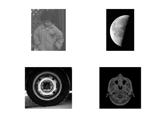
Multiple images in one figure
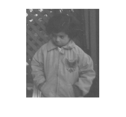
We can display one image in a single figure, but we can also split a figure into a number of regions and display several images there.
figure(1)
imshow(image1);
figure(2)
subplot(2,2,1); imshow(image1);
subplot(2,2,2); imshow(image2);
subplot(2,2,3); imshow(image3);
subplot(2,2,4); imshow(image4);
Colour Images
We will now read a colour image,
image5 = imread ('peppers.png');

figure(3);
subplot(2,2,1)
imagesc(image5)
title('RGB Colour image');
subplot(2,2,2);imagesc(image5(:,:,1))   % Displays Red component
title('Red Channel');

subplot(2,2,3);imagesc(image5(:,:,2))	% Displays Green component
title('Green Channel');

subplot(2,2,4);imagesc(image5(:,:,3))	% Displays Blue component
title('Blue Channel');

colormap (gray)
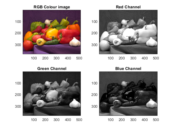
Notice that the individual channels are themselves a greyscale image and it is only when combined that the three create a colour image. Notice also the differences that colours have on the separate channels. This effect is stronger on the red peppers which appear very bright on the red channel and almost black on the blue channel. This means that their colour is formed by mostly red and no blue. On the other hand the green objects are bright on both the red and green showing that they are not purely green. The onion on the foreground is white and appears bright in all channels. Try to look for colourful images, read them in Matlab and display their channels.
Colormap
Some images only contain one colour channel, that is, their dimensions will be [rows x columns x 1]. In other applications, these images would be displayed as grey scale images as there is no direct correspondence of a specific colour for each pixel. When these type of images are displayed in Matlab, there are several ways to display them. Some of these different options will artificially assign colours to the pixels according to some specific colouring rules called "maps" or in the context of Matlab 'colormaps'. In some cases, the maps can provide more contrast that the traditional grey scales. To illustrate these 'colormaps', we will first display only one channel of the fluorescent cells with grey scale:
figure
imagesc(fluorescent_cells(:,:,1))

colormap(gray)
colorbar
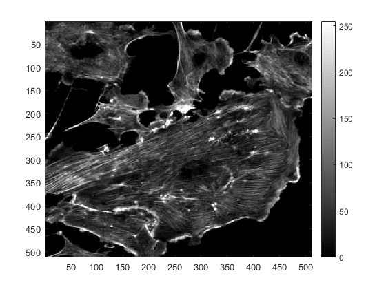
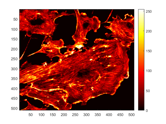
The command 'colormap' specifies the "map" we want to use for this image, in this case a grey scale map, which is displayed in the colour bar on the right, which is added with the command 'colorbar'. To change the map, we simply type a different one, for example:
colormap(hot)
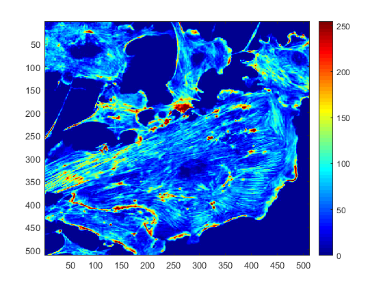
A very typical map, widely used due to its visual discrimination between low and high intensities is the 'jet' map, which uses the colours of the rainbow.
colormap(jet)
There are many different colormaps: 'hot, cool, bone, gray, spring, summer, autumn, winter, hsv, copper', etc. You might want to experiment with a few of these to see which is the best way to display your images. We can even manipulate the colormaps with mathematical functions. The colormaps are predefined matrices with numbers that assign weights for red, green and blue, e.g.
jet
ans =

         0         0    0.5625
         0         0    0.6250
         0         0    0.6875
         0         0    0.7500
         0         0    0.8125
         0         0    0.8750
         0         0    0.9375
         0         0    1.0000
         0    0.0625    1.0000
         0    0.1250    1.0000
         0    0.1875    1.0000
         0    0.2500    1.0000
         0    0.3125    1.0000
         0    0.3750    1.0000
         0    0.4375    1.0000
         0    0.5000    1.0000
         0    0.5625    1.0000
         0    0.6250    1.0000
         0    0.6875    1.0000
         0    0.7500    1.0000
         0    0.8125    1.0000
         0    0.8750    1.0000
         0    0.9375    1.0000
         0    1.0000    1.0000
    0.0625    1.0000    0.9375
    0.1250    1.0000    0.8750
    0.1875    1.0000    0.8125
    0.2500    1.0000    0.7500
    0.3125    1.0000    0.6875
    0.3750    1.0000    0.6250
    0.4375    1.0000    0.5625
    0.5000    1.0000    0.5000
    0.5625    1.0000    0.4375
    0.6250    1.0000    0.3750
    0.6875    1.0000    0.3125
    0.7500    1.0000    0.2500
    0.8125    1.0000    0.1875
    0.8750    1.0000    0.1250
    0.9375    1.0000    0.0625
    1.0000    1.0000         0
    1.0000    0.9375         0
    1.0000    0.8750         0
    1.0000    0.8125         0
    1.0000    0.7500         0
    1.0000    0.6875         0
    1.0000    0.6250         0
    1.0000    0.5625         0
    1.0000    0.5000         0
    1.0000    0.4375         0
    1.0000    0.3750         0
    1.0000    0.3125         0
    1.0000    0.2500         0
    1.0000    0.1875         0
    1.0000    0.1250         0
    1.0000    0.0625         0
    1.0000         0         0
    0.9375         0         0
    0.8750         0         0
    0.8125         0         0
    0.7500         0         0
    0.6875         0         0
    0.6250         0         0
    0.5625         0         0
    0.5000         0         0
Practical Problem: Segmentation of cells
Let's look now at a more complex and realistic example, the segmentation of the fluorescent image previously presented. That image contained a series of cells and their parts were stained in different colours.
To visualise the problem better, let's separate and display the three colour channels:
channel_1 = fluorescent_cells(:,:,1);  % select the first level of the 3D matrix
channel_2 = fluorescent_cells(:,:,2);  % select the second level of the 3D matrix
channel_3 = fluorescent_cells(:,:,3);   % select the third level of the 3D matrix

figure;subplot(1,3,1); imagesc(channel_1)
subplot(1,3,2); imagesc(channel_2)
subplot(1,3,3); imagesc(channel_3)
colormap(jet)
set(gcf,'Position',   [42   378   958   420])
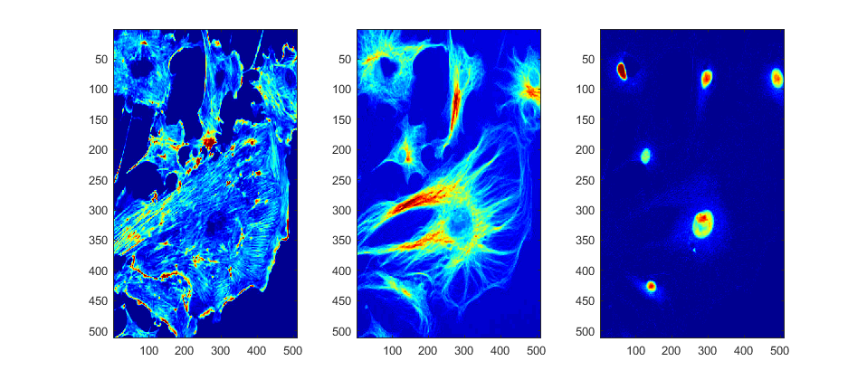
The temptation is to use the blue channel (DAPI) with the nuclei to further process. The selection of another channels may seem weird, BUT Artefacts can affect the results. Segmentation following the nuclei dismisses the shapes of the cells. Let's analyse.
First, let's determine a level for thresholding using Otsu's algorithm
level_1 = 255*graythresh(channel_1);
level_2 = 255*graythresh(channel_2);
level_3 = 255*graythresh(channel_3);
Now, we can segment and display channels separately. (Look carefully)
channel_1B = fluorescent_cells(:,:,1)>level_1;
channel_2B = fluorescent_cells(:,:,2)>level_2;
channel_3B = fluorescent_cells(:,:,3)>level_3;
figure;subplot(1,3,1); imagesc(channel_1B)
subplot(1,3,2); imagesc(channel_2B)
subplot(1,3,3); imagesc(channel_3B)
colormap(gray)
set(gcf,'Position',   [42   378   958   420])
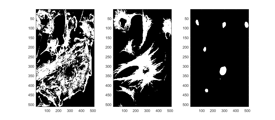
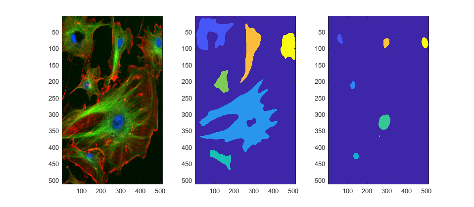
We can safely discard the red channel, it will not help in any way for this segmentation. Now let's label each region, that is, we will assign a unique identifier to each region of connected pixels. Because Channel 2 is a bit more complex, we will smooth it before labelling:
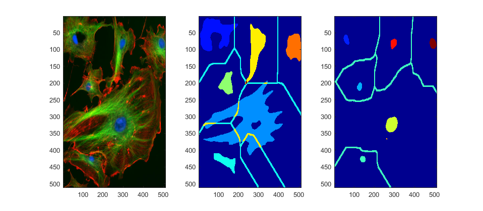
channel_1B = fluorescent_cells(:,:,1)>level_1;
channel_2B = bwlabel(imfilter(fluorescent_cells(:,:,2),fspecial('Gaussian',19*[1 1],7))>level_2);
channel_3B = bwlabel(fluorescent_cells(:,:,3)>level_3);

figure;subplot(1,3,1); imagesc(fluorescent_cells)
subplot(1,3,2); imagesc(channel_2B)
subplot(1,3,3); imagesc(channel_3B)
set(gcf,'Position',   [42   378   958   420])
Compare segmentation with watersheds from the green and blue channels
segmentedBackground     = watershed(1-channel_2B);
segmentedBackground2    = watershed(1-channel_3B);
figure;subplot(1,3,1); imagesc(fluorescent_cells)
subplot(1,3,2); imagesc(channel_2B+3*imdilate((segmentedBackground==0),ones(5)))
subplot(1,3,3); imagesc(channel_3B+3*imdilate((segmentedBackground2==0),ones(5)))
colormap(jet)
set(gcf,'Position',   [42   378   958   420])
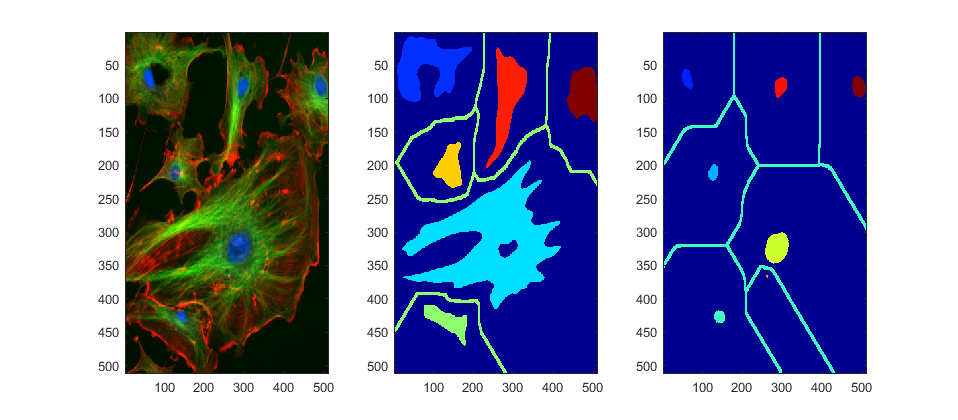
To compare, let's swap segmentations from channels to show which is better
figure
subplot(1,3,1); imagesc(fluorescent_cells)
subplot(1,3,2); imagesc(channel_2B+3*imdilate((segmentedBackground2==0),ones(5)))
subplot(1,3,3); imagesc(channel_3B+3*imdilate((segmentedBackground==0),ones(5)))
colormap(jet)
set(gcf,'Position',   [42   378   958   420])
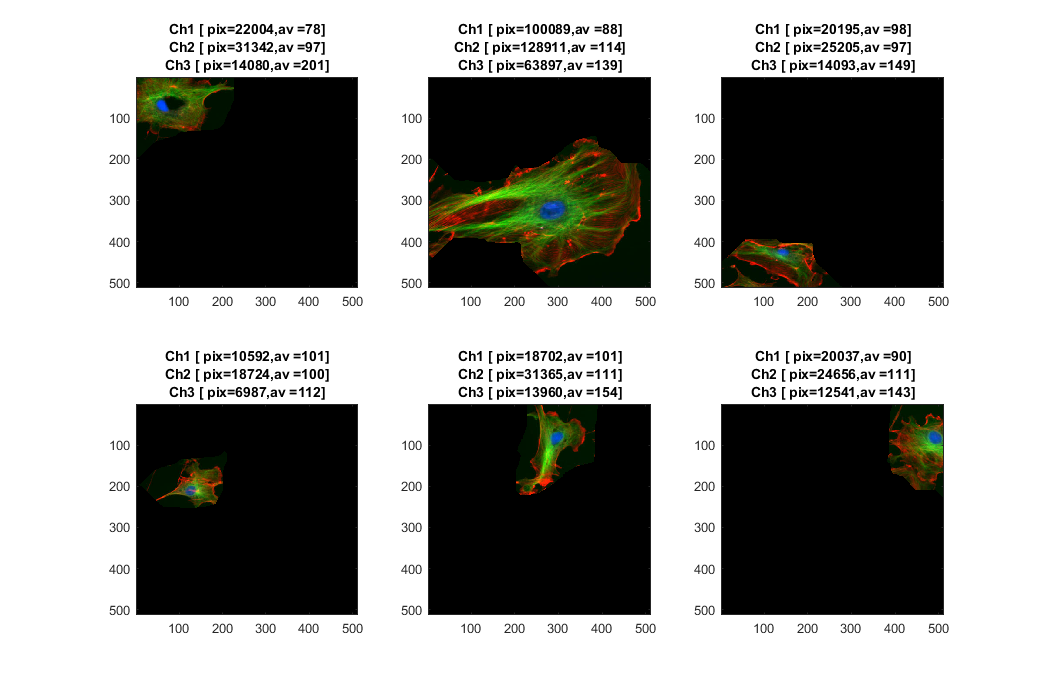
Finally, let's separate each region on the original image. At the same time we can quantify several parameter and display each cell with its metrics.
[rows, columns, channels]= size(fluorescent_cells);
figure
for k=1:6
    subplot(2,3,k)
    currCell = fluorescent_cells.*uint8(repmat(segmentedBackground==k,[1 1 3]));
    currSize = round(sum(sum(currCell(:,:,:)>0)));
    [rr,cc,vv1]  = find(double(currCell(:,:,1)).* channel_1B);
    [rr,cc,vv2]  = find(double(currCell(:,:,2)).*(channel_2B>0));
    [rr,cc,vv3]  = find(double(currCell(:,:,3)).*(channel_3B>0));
    currIntensity1  = round(mean(vv1));
    currIntensity2  = round(mean(vv2));
    currIntensity3  = round(mean(vv3));
    imagesc(currCell)
    title({strcat('Ch1 [ pix=',num2str(currSize(1)),',av = ',...
           num2str(currIntensity1),']');...
           strcat('Ch2 [ pix=',num2str(currSize(2)),',av = ',...
           num2str(currIntensity2),']');...
           strcat('Ch3 [ pix=',num2str(currSize(3)),',av = ',...
           num2str(currIntensity3),']')})
end

set(gcf,'Position',   [  388         108        1043         691])
More options to process images
Here we introduced a few tools to process images like Otsu thresholding, watersheds and labelling. There are many many more techniques, read and try some of these techniques on images: imdilate, imerode, imopen, imclose, strel, bwmorph to start with some.
Reference
This file is part of the material used to introduce Matlab. All these materials are based on the book:
  Biomedical Image Analysis Recipes in Matlab
  For Life Scientists and Engineers
  Wiley, July 2015
  Constantino Carlos Reyes-Aldasoro
  http://eu.wiley.com/WileyCDA/WileyTitle/productCd-1118657551.html
Disclaimer
These files are for guidance and information. The author shall not be liable for any errors or responsibility for the accuracy, completeness, or usefulness of any information, or method in the content, or for any actions taken in reliance thereon.