Tutorial: Introduction to Matlab
Contents
Matlab and matrices
Matlab, MAT rix LAB oratory, is a powerful, high - level language and a technical computing environment, which provides core mathematics and advanced graphical tools for data analysis, visualisation, and algorithm and application development. It is intuitive and easy to use. Many common functions have already been programmed in the main program or on one of the many toolboxes. The Matlab programming environment provides a very large number of advantages, for instance, creating documents. This and other tutorials have been written in Matlab.
Matlab is intuitive and easy to use, but it requires the use of command-line interface. That is, contrary to other software products, which have interfaces and buttons, in Matlab the user needs to type commands to perform tasks.
In MATLAB everything is a matrix, (this is the mantra: everything is a matrix ) and therefore it is a bit different from other programming languages, such as C or JAVA. Matrix operations are programmed so that element - wise operations or linear combinations are more efficient than loops over the array elements. The for instruction is recommended only as a last resource. Once you are in MATLAB, many UNIX commands can be used: pwd, cd, ls, etc. To get help over any command you can type
help
Use the Help browser search field to search the documentation, or
type "help help" for help command options, such as help for methods.
For example
help for
 FOR    Repeat statements a specific number of times.
    The general form of a FOR statement is:

       FOR variable = expr, statement, ..., statement END

    The columns of the expression are stored one at a time in
    the variable and then the following statements, up to the
    END, are executed. The expression is often of the form X:Y,
    in which case its columns are simply scalars. Some examples
    (assume N has already been assigned a value).

         for R = 1:N
             for C = 1:N
                 A(R,C) = 1/(R+C-1);
             end
         end

    Step S with increments of -0.1
         for S = 1.0: -0.1: 0.0, do_some_task(S), end

    Set E to the unit N-vectors
         for E = eye(N), do_some_task(E), end

    Long loops are more memory efficient when the colon expression appears
    in the FOR statement since the index vector is never created.

    The BREAK statement can be used to terminate the loop prematurely.

    See also PARFOR, IF, WHILE, SWITCH, BREAK, CONTINUE, END, COLON.

    Reference page in Doc Center
       doc for
The main window is the 'Desktop', which is subdivided into several sections. The 'Command Window' is where the instructions or commands are written to perform a given task. The user will type the instructions in the 'Command Window'. For example, we can add two numbers 2 and 5 and store the result in the variable 'a' by typing the following in the 'Command Window':
a = 2 + 5
a =

     7
The order of precedence in which the operations are carried out is the following: exponentiation, multiplication/division and then addition and subtraction. This order can be modified by using round brackets. The order is sometimes referred to with the acronyms "BODMAS" or "BIDMAS" which stand for "Brackets, Order of, Division, Multiplication, Addition, Subtraction" and "Brackets, Indices (powers and roots), Division, Multiplication, Addition, Subtraction". Therefore, the following instruction line:
1 + 2 * 3 ^ 4
ans =

   163
is equivalent to:
1 + (2 * (3 ^ 4))
ans =

   163
and is different from
(((1 + 2) * 3) ^ 4)
ans =

        6561
The great advantage of Matlab is to be processing data as matrices, that is, when you save a series of values inside a variable, as a matrix, you should process it as a single entity. In other words, if you are using "for-next loop", there is probably a better way of doing things in Matlab. For example:
x = [ 1 2 3 4 5 6 7 8 9 10 ]
x =

     1     2     3     4     5     6     7     8     9    10
is equivalent to:
x = 1:10
x =

     1     2     3     4     5     6     7     8     9    10
where only initial and final values are specified. It is possible to define the initial and final value and increment (lower limit: increment: upper limit) using the colon operator in the following way:
z = 0 : 0.1 :20;
Both are 1 x 10 matrices. Note that this type of matrices (x,z) would be different from:
y = [1;2;3;4;5;6;7;8;9;10]
y =

     1
     2
     3
     4
     5
     6
     7
     8
     9
    10
or
y=[1:10]'
y =

     1
     2
     3
     4
     5
     6
     7
     8
     9
    10
Both are 10 x 1 matrices. The product x*y would yield the inner product of the vectors, a single value, y*x would yield the outer product, a 10 x 10 matrix, while the products x*x and y*y are not valid because the matrix dimensions do not agree. If element-to-element operations are desired then a dot "." before the operator can be used, e. g. x.*x would multiply the elements of the vectors:
x*y
ans =

   385
The following line will produce an error. To isolate errors you can use the commands 'try' and 'catch' like this
try
    x*x
catch errorDescription
    disp('Error, the dimensions of the matrices do not agree, it is like adding apples and pears');
end
Error, the dimensions of the matrices do not agree, it is like adding apples and pears
The error message above is not the one that Matlab would provide.
In the previous lines we have used an advance feature of programming languages called "exception handling" or "error catching" which is designed to deal with errors. Matlab handles exceptions in the following way: all the lines of code that are placed inside a block delimited by the statements 'try' and 'catch' (only one line in this case) are under a special consideration: if errors occur inside this block, Matlab will not return an error message or crash a process if it was run within a function or script. Instead, Matlab will "catch" the exception and record the error in the variable placed immediately after the command 'catch' ('errorDescription'), and will execute instead the statements in the block delimited by 'catch' and 'end'. In this case we only displayed an error message, but in other cases it is possible to indicate an alternative commands.
The error messages in Matlab in some cases may seem a bit cryptic, but it is important to read them to understand the possible sources of any errors. In this example, the inconsistent dimensions of the two matrices to be combined created the error. We can investigate the variable 'errorDescription' of our previous example by typing the name of the variable on the Command Window like this:
errorDescription
errorDescription =

  MException with properties:

    identifier: 'MATLAB:innerdim'
       message: 'Incorrect dimensions for matrix multiplication. Check that the number of columns in the first matrix matches the number of rows in the second matrix. To perform elementwise multiplication, use '.*'.'
         cause: {0×1 cell}
         stack: [5×1 struct]
    Correction: []
Let's continue with other multiplications, to avoid the error previously described due to the dimensions, we can use the "dot product" in which each element of one matrix multiplies one element of the other matrix like this
x.*x
ans =

     1     4     9    16    25    36    49    64    81   100
Notice that this is equivalent of squaring each element of the matrix. Notice also that the order in which you multiply matrices matters, i.e. x*y is not the same as y*x, try this:
y*x
ans =

     1     2     3     4     5     6     7     8     9    10
     2     4     6     8    10    12    14    16    18    20
     3     6     9    12    15    18    21    24    27    30
     4     8    12    16    20    24    28    32    36    40
     5    10    15    20    25    30    35    40    45    50
     6    12    18    24    30    36    42    48    54    60
     7    14    21    28    35    42    49    56    63    70
     8    16    24    32    40    48    56    64    72    80
     9    18    27    36    45    54    63    72    81    90
    10    20    30    40    50    60    70    80    90   100
2D Matrices
A 2D matrix can be obtained by typing a semicolon to separate between rows:
mat = [1 2 3 4;2 3 4 5;3 4 5 6;4 5 6 7];
Notice that the final semicolon (;) inhibits the echo to the screen. Any individual value of the matrix can be read by typing (without the semicolon):
mat (2,2)
ans =

     3
There are different ways to investigate or look into the values of a matrix. Perhaps the simplest way is to type the name of the variable in the command line, and press enter. Since there is no semicolon at the end of the line, the values of the matrix will be echoed into the Command Window. This method is not very useful for matrices with many rows and columns. For large matrices it is better to use the "Variable Editor" which looks like an Excel spread sheet with the values of the matrix. To open a matrix into the Variable Editor you can use the command 'openvar' followed by the variable of interest like this:
openvar x
Combining matrices
As you have noticed by now, matrices are not restricted to have only one column or one row. Matrices can have many dimensions. Indeed, an image is a special case of a matrix, as we will see later. You can create a matrix with several rows and columns by typing them directly; each row is started with a semicolon:
matrix_1 = [1 2 3 4;2 3 4 5;3 4 5 6;4 5 6 7; 9 9 9 9];
You can create a matrix by using other matrices as with the previous examples (z7 or z8), but you need to be careful with the dimensions of the elements that will form a new matrix. As an example, we can form two new matrices based on 'matrix_1', first by concatenating them horizontally and then vertically like this:
matrix_2                = [matrix_1 matrix_1]

matrix_3                = [matrix_1;matrix_1]
matrix_2 =

     1     2     3     4     1     2     3     4
     2     3     4     5     2     3     4     5
     3     4     5     6     3     4     5     6
     4     5     6     7     4     5     6     7
     9     9     9     9     9     9     9     9


matrix_3 =

     1     2     3     4
     2     3     4     5
     3     4     5     6
     4     5     6     7
     9     9     9     9
     1     2     3     4
     2     3     4     5
     3     4     5     6
     4     5     6     7
     9     9     9     9
You can also combine matrices and apply mathematical operations at the same time. For example, we can take one matrix, apply different mathematical operations to it and store all results in a new matrix. Let's illustrate this example by modifying 'matrix_1' with several operations like this:
matrix_4                = [matrix_1  matrix_1+20 matrix_1*3   ;...
                           matrix_1./2  sqrt(matrix_1) matrix_1.^2 ]
matrix_4 =

  Columns 1 through 7

    1.0000    2.0000    3.0000    4.0000   21.0000   22.0000   23.0000
    2.0000    3.0000    4.0000    5.0000   22.0000   23.0000   24.0000
    3.0000    4.0000    5.0000    6.0000   23.0000   24.0000   25.0000
    4.0000    5.0000    6.0000    7.0000   24.0000   25.0000   26.0000
    9.0000    9.0000    9.0000    9.0000   29.0000   29.0000   29.0000
    0.5000    1.0000    1.5000    2.0000    1.0000    1.4142    1.7321
    1.0000    1.5000    2.0000    2.5000    1.4142    1.7321    2.0000
    1.5000    2.0000    2.5000    3.0000    1.7321    2.0000    2.2361
    2.0000    2.5000    3.0000    3.5000    2.0000    2.2361    2.4495
    4.5000    4.5000    4.5000    4.5000    3.0000    3.0000    3.0000

  Columns 8 through 12

   24.0000    3.0000    6.0000    9.0000   12.0000
   25.0000    6.0000    9.0000   12.0000   15.0000
   26.0000    9.0000   12.0000   15.0000   18.0000
   27.0000   12.0000   15.0000   18.0000   21.0000
   29.0000   27.0000   27.0000   27.0000   27.0000
    2.0000    1.0000    4.0000    9.0000   16.0000
    2.2361    4.0000    9.0000   16.0000   25.0000
    2.4495    9.0000   16.0000   25.0000   36.0000
    2.6458   16.0000   25.0000   36.0000   49.0000
    3.0000   81.0000   81.0000   81.0000   81.0000
Addressing a matrix
In many cases, especially when you are dealing with large matrices as the ones that will correspond to an image, it is important to be able to obtain or modify only a subset of the values of the matrices. Imagine for instance, (a) that you want to zoom to a certain region of an image, (b) you want to subsample your image by discarding odd rows and keeping the even ones, or (c) you may want to select only those experiments for which a certain concentration of cells is larger than a predefined value. All these examples are very easy to do in Matlab by "addressing" a matrix. In other enviroments this is sometimes called "slicing", "dicing", and when it is more involved it can also be known "wrangling" or "munging", which refers to re-arranging data from one format into another format.
The simplest cases of addressing a matrix are to obtain values that are in special positions of the matrix. For example, to obtain a value or range of values of the previously defined matrices you need to type the values between brackets after the name of the matrix with the following format (row(s), column(s)).
matrix_1(2,2)
matrix_2(2:3,1:3)
matrix_3(1:2:end,:)
ans =

     3


ans =

     2     3     4
     3     4     5


ans =

     1     2     3     4
     3     4     5     6
     9     9     9     9
     2     3     4     5
     4     5     6     7
The previous examples show three ways of addressing a matrix. First, a single element is retrieved; the value stored in the second row and second column. The second example retrieves the values stored in the second to third row and first to third column. The third example uses the colon operator described previously to address all the odd rows, the shorthand notation '1:2:end' can be translated into words as: "rows that start at 1, increment by 2 until rows finish". The columns also use a short hand, the colon operator on its own ":" is equivalent to writing '1:end' or "take all columns of the matrix_3".
In the same way that the addressing of the matrix can be used to retrieve values, it can also be used to change the values of a matrix. For instance, if we would like to change to zero the first column of a matrix we could type:
matrix_1(:,1) = 0
matrix_1 =

     0     2     3     4
     0     3     4     5
     0     4     5     6
     0     5     6     7
     0     9     9     9
or change all the values of the first row to -1:
matrix_2(1,:) = -1
matrix_2 =

    -1    -1    -1    -1    -1    -1    -1    -1
     2     3     4     5     2     3     4     5
     3     4     5     6     3     4     5     6
     4     5     6     7     4     5     6     7
     9     9     9     9     9     9     9     9
To change a specific region, for example, to leave the border elements unchanged and set all the inside elements of the matrix to zero we could type:
matrix_3(2:end-1,2:end-1) = 0
matrix_3 =

     1     2     3     4
     2     0     0     5
     3     0     0     6
     4     0     0     7
     9     0     0     9
     1     0     0     4
     2     0     0     5
     3     0     0     6
     4     0     0     7
     9     9     9     9
or the opposite, to set the boundary elements to zero and leave the central values unchanged:
matrix_4([1 end],:)     = 0;
matrix_4(:,[1 end])     = 0
matrix_4 =

  Columns 1 through 7

         0         0         0         0         0         0         0
         0    3.0000    4.0000    5.0000   22.0000   23.0000   24.0000
         0    4.0000    5.0000    6.0000   23.0000   24.0000   25.0000
         0    5.0000    6.0000    7.0000   24.0000   25.0000   26.0000
         0    9.0000    9.0000    9.0000   29.0000   29.0000   29.0000
         0    1.0000    1.5000    2.0000    1.0000    1.4142    1.7321
         0    1.5000    2.0000    2.5000    1.4142    1.7321    2.0000
         0    2.0000    2.5000    3.0000    1.7321    2.0000    2.2361
         0    2.5000    3.0000    3.5000    2.0000    2.2361    2.4495
         0         0         0         0         0         0         0

  Columns 8 through 12

         0         0         0         0         0
   25.0000    6.0000    9.0000   12.0000         0
   26.0000    9.0000   12.0000   15.0000         0
   27.0000   12.0000   15.0000   18.0000         0
   29.0000   27.0000   27.0000   27.0000         0
    2.0000    1.0000    4.0000    9.0000         0
    2.2361    4.0000    9.0000   16.0000         0
    2.4495    9.0000   16.0000   25.0000         0
    2.6458   16.0000   25.0000   36.0000         0
         0         0         0         0         0
Notice that it is possible to use the 'end' operator as a value. This is very useful when you do not know the dimensions of the matrix, for instance when you are going to process images of different sizes.
There are two more important issues to know regarding the addressing of a matrix. First, it is possible to copy parts of a matrix by addressing the matrix to be copied, for instance:
matrix_5 = matrix_1(1:end,2:3);
This function will be handy when dealing with images; for instance a colour image, and we are only interested in the blue channel, or when we want to zoom into a special section of the image.
In the previous examples we have enlarged matrices by combining them, in this way, we have added elements, appended them to non-existent places of the matrix. We can create matrices of any dimensions by assigning just one value to a position, for example, if we would like to create a matrix with 500 rows, 200 columns and three levels (a three dimensional matrix, such as an image with three colour channels) we only need to assign a value, usually a zero) to the last position of the matrix:
matrix_6(500,200,3) = 0;
We can extend already existing matrices in the same way:
matrix_1(10,15,4) = 0;
Second, to remove elements of a matrix, we need to declare those elements as 'empty'. An empty matrix is declared in Matlab as two square brackets and nothing between them ("[ ]"), thus to remove the first column of a matrix, we could type:
matrix_2 (:,1) = []
matrix_2 =

    -1    -1    -1    -1    -1    -1    -1
     3     4     5     2     3     4     5
     4     5     6     3     4     5     6
     5     6     7     4     5     6     7
     9     9     9     9     9     9     9
To remove the last row of the same matrix we would type the following code into the Command Window:
matrix_2 (end,:) = []
matrix_2 =

    -1    -1    -1    -1    -1    -1    -1
     3     4     5     2     3     4     5
     4     5     6     3     4     5     6
     5     6     7     4     5     6     7
It should be apparent by now that the size of the matrices can be important in many cases, either to know the dimensions so that the matrix can be addressed, or to prepare other matrices that will be used in future commands. To obtain the dimensions of a matrix we use the command 'size' followed by the name of the variable we want to measure the size. It is possible to echo the answer to the Command Windows, but we can also store it in new variables in case we need that value later on. As it was said before, it is convenient to use sensible names for our variables, for example:
[numberRows,numberColumns] = size (matrix_2);
If you are only interested in one dimension of a matrix, you can specify that dimension by writing down the number of the dimension after the name of the matrix like this:
[numberColumns]         = size (matrix_2,2);
[numberLevels]          = size (matrix_2,3);
Mathematical functions can be used over the defined matrices, for example:
s1 = sin (z);
A column or line of a matrix can be obtained from another one:
s2(1,:) = -s1/2;
s2(2,:) = s1;
s2(3,:) = s1 * 4;
Let's observe the plot of one of the matrices previously generated:
plot(s1);
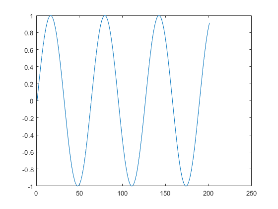
The graph shows a sine curve that starts in zero, oscillates between [-1,+1] and spans 201 time points. The horizontal axis is defined by the location of the values of the matrix from 1 to 201. However, we know that these observations were done between 0 and 20, therefore we would like our plot to show these values in that range. To combine the time and the values of the observations in one single plot, we need to indicate this by passing two variables as arguments to the command 'plot'; first the variable that will correspond to the horizontal axis and second the one that corresponds to the vertical axis, e.g
plot(z,s1);
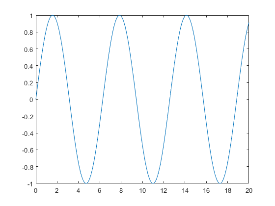
Notice that the graphic is very similar but now the values of the horizontal axis go from 0 to 20 and there is no empty space on the right hand side of the graph. By default Matlab draws the plot with a continuous blue line between points. However, we can easily modify this by adding a third argument to the command 'plot'. For example, we can draw the line in red, with round markers to each point, like this:
plot(z,s1,'r-o');
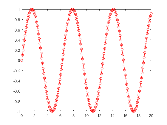
The third argument 'r-o' is the shorthand notation to specify a red colour ('r'), a continuous line ('-') and round markers ('o'). There is a wide range of possible colours, lines and markers to be used. These are especially useful when plotting several lines in the same figure, for example:
plot(z,s1,'r-.o',z,abs(s1),'b-x');
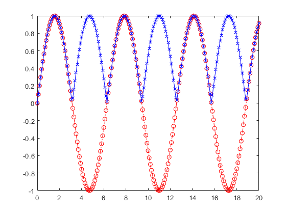
Notice that it is possible to combine plots by applying functions or operations directly on the plotting lines:
Two dimensional graphs are also very easy to display, for instance:
mesh(s2);
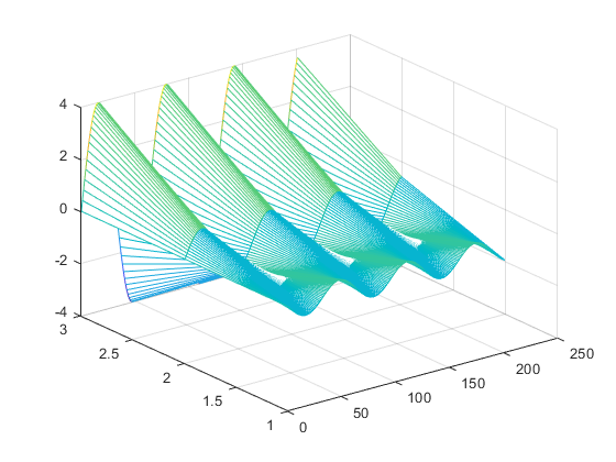
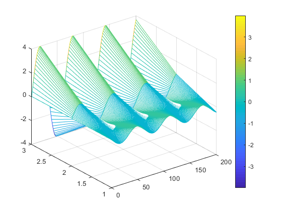
creates a 'mesh', that is a series of lines connecting between the points of the 2D data set. To see how the colour corresponds to the vertical axis we can add a colour bar like this:
colorbar
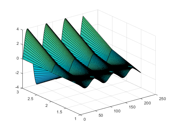
There are other nice options to display data in 3 dimensions (from a 2D matrix, for instance a ribbon
ribbon(s2')
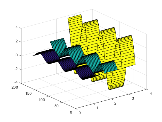
Notice that the direction of the data determines the number of ribbons, i.e. look at these ribbons:
ribbon(s2)
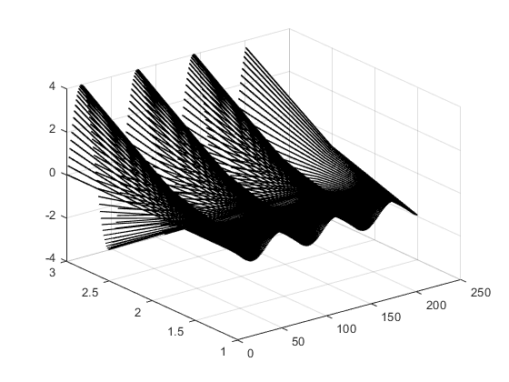
surf(s2)
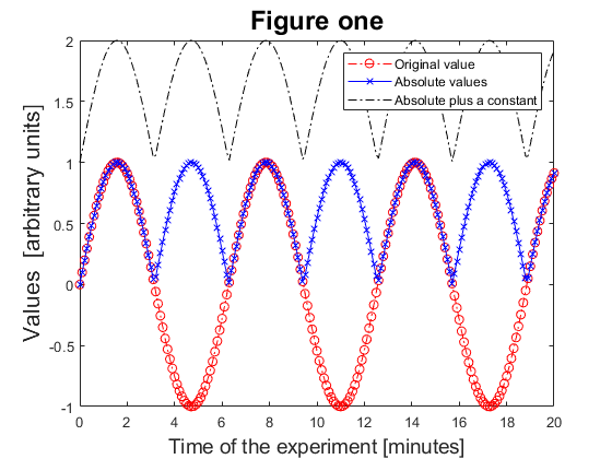
One important aspect of figures is to be descriptive, and for that we can add labels on the axes, titles and legends. We can do that with the following commands: 'xlabel', 'ylabel' and 'zlabel' to add labels to each of the coordinate axis, in this case we do not have a z-axis. Titles are inserted with the command 'title' and legends with 'legend' like this:
plot(z,s1,'r-.o',z,abs(s1),'b-x',z,1+ abs(s1),'k-.');

xlabel('Time of the experiment [minutes]','fontsize',14);
ylabel('Values  [arbitrary units]','fontsize',16);
title('Figure one','fontsize',18);
legend('Original value', 'Absolute values', 'Absolute plus a constant');

Notice that it is possible to have different font sizes for each of the labels that we add to the image. It should be clear that the commands in Matlab have names that should be fairly intuitive to use. If we want to add a grid we use the command 'grid' and turn it 'on' like this:
grid on;

To remove the grid, the command has to be followed by 'off' like this:
grid off
To erase all the content of a figure, we use the command 'clf', which stands for "clear figure". Or if we want to close the figure, we type 'close' followed by the number of the figure, in this case 1 like this 'close (1)' or alternatively we pass the handle to the current figure which is 'gcf' (get current figure) like this
close gcf
If we want to erase variables that we have created we use 'clear' followed by the name of the variable. To erase every variable (with caution!) simply type 'clear' and press enter:
clear
More help
In your own time use help to find out more about some of the following Matlab commands:
sign, subplot, abs, imshow, surf, colormap,
sum, cumsum, fix, round, subplot, whos,
zeros, ones, rand, randn, real, abs.
There are many toolboxes with specialised functions, try:
  help images %	Image processing toolbox.
  help signal %	Signal processing toolbox.
  help stats	 %	Statistics toolbox
  help nnet	 %	Neural networks toolbox
To find out which toolboxes you have installed type 'ver'
Reference
This file is part of the material used to introduce Matlab. All these materials are based on the book:
  Biomedical Image Analysis Recipes in Matlab
  For Life Scientists and Engineers
  Wiley, July 2015
  Constantino Carlos Reyes-Aldasoro
http://eu.wiley.com/WileyCDA/WileyTitle/productCd-1118657551.html
Disclaimer
These files are for guidance and information. The author shall not be liable for any errors or responsibility for the accuracy, completeness, or usefulness of any information, or method in the content, or for any actions taken in reliance thereon.