|
|||||||
|
||||||||
It is possible to create new raster surfaces by selecting Create New Raster...
from the Edit menu. You will be presented with a dialogue window
allowing the bounds and resolution of the new surface to be changed. The default settings create
a raster with 100 rows and 100 columns.
 Creating a polynomial surface.
The new raster can be either 'blank' containing only zeros, a polynomial expression, or a fractal surface with a user-defined fractal dimension. Fractal surfaces can be useful for modelling and simulation or terrains.
For modelling and simulation purposes it is sometimes useful to create artificial surfaces with known
characteristics. By selecting Polynomial from the Create New Raster window,
you can define functions with the following variables and functions.
| Expression | Explanation |
x | the x position of each raster cell. x is scaled to be +- nCols/2, where nCols is the number of columns in the raster |
y | the y position of each raster cell. y is scaled to be +- nRows/2, where nRows is the number of rows in the raster |
z0 | the value of any given cell in the currently selected raster. This will only be meaningful if a raster already exists; if it does not, z0 will always return 0. |
z1 | the value of any given cell in the secondary raster (typically the 'drape'). This will only be meaningful if a drape already exists; if it does not, z1 will always return 0. |
+, -, *, /, ^ | Addition, subtraction, multiplication, division and power operators. |
cos(), sin(), tan() | trigonometrical functions. Expects angles to be given in radians (to convert from
degrees into radians multiply by p/180 or 0.01745329). Values of infinity (e.g.
tan(p/2)) are returned as 0. |
acos(), asin(), atan() | inverse trigonometrical functions. Returns values in radians (to convert from radians into degrees multiply by 180/p or 57.2957795). Values outside of the range of +-1 supplied to these functions will return a value of 0. |
sqrt() | Square root. If the value given to the function is negative, the function will return a 0. |
ln() | Natural logarithm (to base e). If the value given to the function is <=0, the function will return a zero. |
() | Brackets to control the order of evaluation. |
| Example | Explanation |
x+y | Creates a plane sloping from bottom right to top left. |
0 - (x^2 + y^2) | Creates a convex-up dome. |
z0-z1 | Creates a difference map of the differences between the surface and drape. |
100 - sqrt((x*y*sin(x*y/200) * cos(y/30))+(x^2+y^2)) | Complex polynomial (peak with 8 radial valleys) |
Expressions that are incorrectly specified (e.g. using unknown functions, or failure to close brackets), are highlighted in the edit window preventing it from being closed.
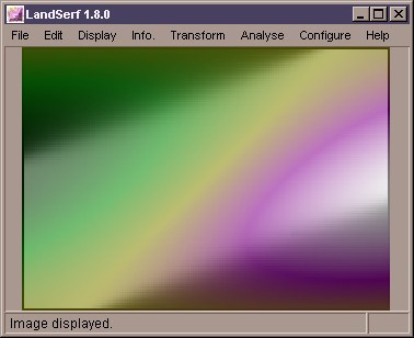 A polynomial surface.
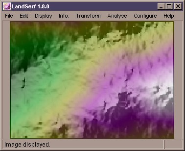 A combined polynomial and fractal surface.
By selecting Fractal from the Create New Raster window, more realistic terrain surfaces may be
created for modelling and simulation purposes. The roughness of such surfaces can be controlled by entering a fractal dimension
between 2.0 (smooth) and 3.0 (very rough). Typical landscapes have fractal dimensions of around 2.1.
These may also be combined with smoother polynomial surfaces, as shown in the figures above. This can be achieved by creating a
fractal surface, changing processing to 'drape', creating a polynomial surface and finally creating a new polynomial as
z0+z1, thus combining the two simulated fields.
Existing rasters or vectors can be edited in much the same way by selecting
Edit Raster Information... or Edit Vector Information....
Here you are able to change the spatial bounds, the title and notes associated with the data. In
the case of raster data, it is possible to 'subset' the surface by specifying new spatial bounds
that lie within the existing ones. These may be specified either by typing in the new coordinates
in the North, South, East
and West fields, or by dragging the mouse over the sub-region of
interest. The Extract Subset of Raster item must then be checked.
If you wish to change the resolution of an existing raster, the new values should be entered in
the E-W Res and N-S Res fields and the
Interpolate to new resolution item must be checked. LandSerf will
then reinterpolate the elevation model to the desired resolution. This technique can be used to
remove 'steps' in a coarse DEM, or to provide an optimal sampling strategy for DEMs that are too
large for effective processing.
 Raster transformation.
A series of simple transformations can be applied to any raster by selecting Transform Raster Values...
from the Transform menu. Raster values are scaled by the value in the
Scale field, translated 'up' or 'down' by the Translate
value or rounded to the nearest Round value. The elevation model can
also be 'flooded' such that all elevations below the value in the Flood
field will be assigned that height. Transformations are only applied if the relevant check box is
selected.
 Triangulation options.
A raster DEM can be converted into a vector Triangulated Irregular Network (TIN) be selecting
DEM to TIN... from the Transform
menu. You will then be presented with a dialogue window asking for various triangulation options.
To control the number of triangles produced by the process, either specify the number explicitly
and select the relevant check box, or specify some error criterion. The error (either average as
specified by the Root Mean Squared Error, or the maximum error) represents the difference in
elevation between any point on the original DEM and its elevation in the TIN. The smaller the error
specified, the greater the number of triangles required in the network. A visualisation of the spatial
pattern of errors can be produced by selecting Create Error Surface
from the dialogue box.
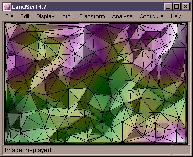 A fractal TIN.
The triangulation process works by successively adding triangles to the network until either any of the selected error criteria are met, or the maximum number of triangles is reached (if specified). Calling the DEM to TIN transformation on successive occasions will add triangles to the existing network rather than recreate a new network from scratch. In this way it is possible to view the network while it is being built.
It is also possible to convert a given TIN back into a DEM. This is achieved by selecting
TIN to DEM... from the Transform menu.
LandSerf will apply a planar interpolation of the triangle network which tends to produce a surface
composed of flat facets. If necessary, these can be smoothed using Quadratic Interpolation (see
the Analysis chapter for details).
 Contours threaded through fractal surface.
Finally, it is possible to create a contour coverage of a given DEM by selecting DEM to contours... from the
Transform menu. Once selected, you can control the contour interval and the elevation of the lowest contour.
For DEMs with large flat areas (e.g. sea around an island), more useful results are produced when a contours do not coincide
with the elevation of the extended flat region. The Grid width option controls the resolution at which DEM cells
are sampled in order to thread contour lines. A value of 1 will sample every DEM cell and produce the most detailed contour
lines; larger values will be faster and will generalise the resulting contours.
