

All spatial objects used by LandSerf are fully georeferenced. This allows rasters and vectors to be
co-registered when overlaying one on the other. To display this information, select the relevant objects from
the thumbnail view and select either Info->Summary Info or the
![]() button. This displays the title,
bounds, map projection information, notes and colour table associated with the spatial object (see figure below).
This information may be changed by selecting the relevant item from the
button. This displays the title,
bounds, map projection information, notes and colour table associated with the spatial object (see figure below).
This information may be changed by selecting the relevant item from the Edit menu.
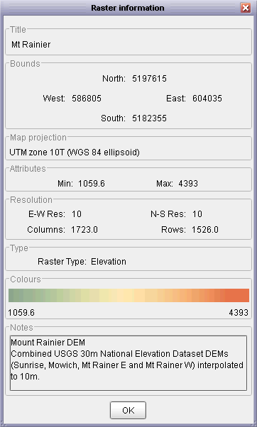 Spatial object summary information.
Univariate statistics for a raster can be calculated by selecting the Info->Statistical summary
menu item. This will calculate measures of average, dispersion and spatial autocorrelation (local roughness).
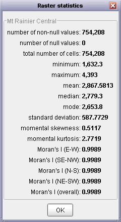 Raster statistical summary.
More detailed information about raster and vector attributes can be found by querying the spatial object
interactively with the mouse. To do this, place LandSerf in Query Mode by either selecting the
Info->Query Map menu item or by toggling the
![]() button. By moving the mouse
over the main LandSerf display, location and attribute associated with the current mouse position will
be displayed at the bottom of the main window. A permanent record of these query results are displayed
in the LandSerf console and recorded in the LandSerf log file
(see Chapter 1 - Introduction).
If a spatial object is associated with an attribute table (see Chapter 3 - Creating,
Editing and Transforming Data for more details), the value displayed will be determined by the
active attribute selected from that table. This allows textual as well numerical values to be
displayed. If a secondary raster or primary vector is selected, clicking on a location while in query mode will display
both these attributes too.
button. By moving the mouse
over the main LandSerf display, location and attribute associated with the current mouse position will
be displayed at the bottom of the main window. A permanent record of these query results are displayed
in the LandSerf console and recorded in the LandSerf log file
(see Chapter 1 - Introduction).
If a spatial object is associated with an attribute table (see Chapter 3 - Creating,
Editing and Transforming Data for more details), the value displayed will be determined by the
active attribute selected from that table. This allows textual as well numerical values to be
displayed. If a secondary raster or primary vector is selected, clicking on a location while in query mode will display
both these attributes too.
To query more than one raster cell value at a time, cross-sectional profiles can be displayed by selecting
either the Info->Profile menu item or the
![]() button. By clicking somewhere on the main raster display and dragging
the mouse to another location, linear cross-sections are displayed in the profile window. The labels
along the X-axis give the distance from the first point in the profile in ground units. The number of
sample points along the profile can be controlled by the slider at the bottom of the profile window.
button. By clicking somewhere on the main raster display and dragging
the mouse to another location, linear cross-sections are displayed in the profile window. The labels
along the X-axis give the distance from the first point in the profile in ground units. The number of
sample points along the profile can be controlled by the slider at the bottom of the profile window.
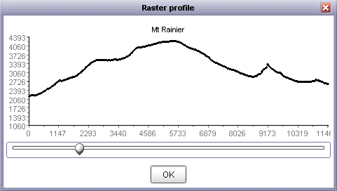 Interactive elevation profile output.
It is also possible to query various surface parameter values interactively using the mouse. To do this,
make sure a DEM is displayed and select the Info->Multi-scale query... from the Info menu.
This opens a dialogue box asking for the window scale and parameter type to be selected (see
Chapter 7 - Performing Analysis on Surfaces for more details on these parameters).
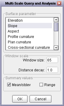 Multi-scale query options.
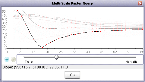
By dragging the mouse over the main display, output similar to that shown below is produced. The graph
shows the value of the selected parameter (slope, curvature, feature type etc.) on the vertical axis,
and the spatial extent over which the parameter was measured on the horizontal axis. Thus the curve produced
shows how the given parameter varies with scale.
 Interactive multi-scale query output with negative curve accumulation.
The numeric values at the bottom of the window represent the location of the point being queried and
either the mean and standard deviation of the queried parameter over all scales, or its minimum and
maximum vales, depending on what was selected in the Query Options window. If aspect is
selected as the parameter to query, the circular mean and standard deviation are displayed. If categorical
parameters such as feature type are selected, the mode and entropy are displayed. The higher the standard
deviation or entropy, the greater the scale dependency of the measure.
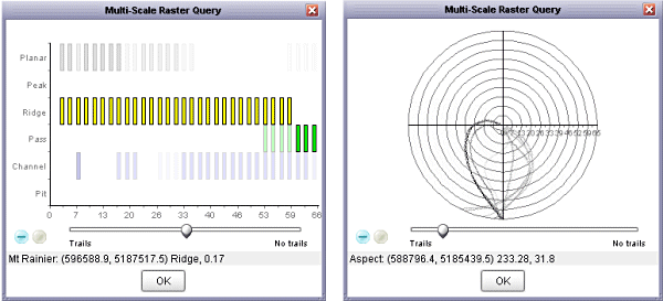 Interactive multi-scale output of feature type (left) and aspect (right) queries.
Curves are updated dynamically as the mouse is dragged over the surface. Old curves can be left on the
display by moving the slider towards the Trails end. Leaving old curves on the graph allows
the spatial variation in scale dependency to be shown as a query area is moved over a surface. They way
in which old query curves are displayed can be controlled by toggling between the
![]() and
and
![]() buttons. Positive accumulation
means that as successive lines are drawn over the same location, their representation becomes darker.
Negative accumulation means that as curves are replaced with newer ones, they become progressively
lighter. Pressing the
buttons. Positive accumulation
means that as successive lines are drawn over the same location, their representation becomes darker.
Negative accumulation means that as curves are replaced with newer ones, they become progressively
lighter. Pressing the ![]() button will
clear the current graph display.
button will
clear the current graph display.
To compare the values of two rasters, select the Info->Scatterplot menu item or the
![]() button. This will plot the
currently selected primary raster as the independent variable on the horizontal axis, and the secondary
surface as the dependent variable on the Y-axis axis. The number of samples taken from the two rasters can be
controlled with the slider.
button. This will plot the
currently selected primary raster as the independent variable on the horizontal axis, and the secondary
surface as the dependent variable on the Y-axis axis. The number of samples taken from the two rasters can be
controlled with the slider.
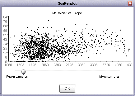 Scatterplot output comparing elevation (X) and slope (Y)
To examine the frequency distribution of a raster, select either the Info->Histogram menu item
or the ![]() button. This plots a
frequency histogram of the primary raster using its colour table. The class width of the histogram can be
controlled via the slider at the bottom of the graph. Moving the slider to the right increases the width
of each class and therefore the total number of classes. Surfaces that contain large flat areas such as
lakes or sea can produce histograms dominated by the elevation of the flat region. Such areas can be
removed from analysis by ticking the
button. This plots a
frequency histogram of the primary raster using its colour table. The class width of the histogram can be
controlled via the slider at the bottom of the graph. Moving the slider to the right increases the width
of each class and therefore the total number of classes. Surfaces that contain large flat areas such as
lakes or sea can produce histograms dominated by the elevation of the flat region. Such areas can be
removed from analysis by ticking the Ignore values at box and supplying an appropriate value.
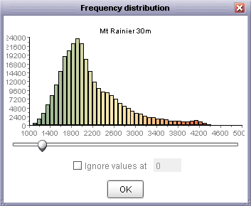 Frequency histogram of elevation surface
Many DEMs exhibit artifacts of the original contour lines that were interpolated to create the surface
model. This can sometimes be detected by examining the frequency distribution of elevation values. For
example, a DEM derived from 10m contour lines may show higher frequencies of 10m, 20m, 30m... elevations
than 5m, 15m, 25m... elevations. This effect can be visualised by plotting the frequency histogram not
of the elevation values directly, but the modulus (remainder) to the base of the suspected contour
interval. To do this, select the Info->Hammock plot menu item. DEMs that show this
effect will result in a 'U' shaped hammock plot. DEMs that do not show this effect will typically show
a rectangular distribution.
Note that large flat areas (e.g. lakes or sea) will significantly affect the hammock distribution,
so as with the frequency histogram, a user-defined value can be ignored in the calculation. The modulus
value used for calculation of the plot defaults to 10, but can altered by moving the slider.
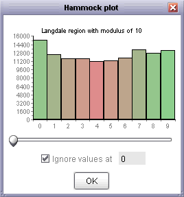 Hammock plot of elevation surface showing bias towards multiples of 10