This is an old version of LandSerf. For the latest release please visit www.landserf.org

LandSerf 2.2 Tutorial

This simple tutorial describes the process that you might go through when using LandSerf for terrain analysis. You can follow the steps using the sample data provided with LandSerf or you can adapt it to use with your own elevation data.

Step 1 - Importing an elevation model.
Step 2 - Georeferencing Information
Step 3 - Displaying the surface.
Step 4 - Attaching metadata to Rasters.
Step 5 - Simple morphometric analysis.
Step 6 - Advanced morphometric analysis.

You can start LandSerf by using one of the following methods:

Selecting it from the Start menu (Windows)
Click on the LandSerf icon on the desktop (Windows)
Click on landserf.command in the Applications folder (MacOSX)
running landserf.sh from the command line (UNIX/Linux/MacOSX)
run or click on landserf.bat (Windows)

Step 1 - Importing an elevation model.

The first stage of any terrain analysis is to import a digital model of the land surface to analyse. Much of LandSerf's functionality concerns processing Digital Elevation Models (DEMs) so we will concentrate on that here. A DEM is simply a matrix of elevation values that describes the height of some surface at regular spatial intervals.

For this tutorial, we shall import a DEM from the United States' National Elevation Dataset representing part of the Columbia River area in Washington state. You may wish to substitute an alternative area of interest (in which case you can find further details on importing data into LandSerf). The DEM we wish to import for this exercise is taken from the United States Geological Survey (USGS) Seamless data server that allows data to be selected from user-defined regions of the American continent. The data are provided in ArcGIS Binary Interleaved Layer (BIL) format and can be found in the data sub-directory of the LandSerf installation.

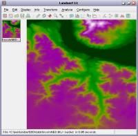Figure 1

To import the elevation file:

Select either the File->Open... menu or the button.
In the drop-down menu labelled Files of Type, select the ArcGIS Binary Image (.bil) format.
Use the dialogue window to navigate to the data sub-directory of the LandSerf directory (if you have used this version of LandSerf before, the file dialogue will default to the last directory you have used). Select the file lincolnNED.bil to load this file.

You should see a square image of the elevation surface as shown in Figure 1. The smaller thumbnail image on the left-hand side of the LandSerf window acts as an 'index' entry. Every time a new object is loaded into LandSerf, a new thumbnail will be added to this index.

Step 2 - Georeferencing Information.

The elevation model provided by the USGS is currently georeferenced using global latitude and longitude values. That is, each of the four corners of the surface are associated with particular locations on the earth's surface. To find out these values we can view the georeferencing information by doing the following:

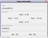LincolnNED global georeferencing information

Figure 2

Select either the Info->Summary Info menu item or the button. This should produce a new window, part of which is shown in Figure 2.

The problem with using global latitude and longitude values for analysis is that they do not correspond to fixed distances on the ground. One degree of longitude will vary in length depending on the latitude of the measurement. It is therefore useful for us to be able to reproject the surface onto a planar coordinate system where there is a fixed scale between the units used and measurements on the ground. For this tutorial, we will firstly store the fact that the imported file uses global latitude/longitude coordinates, then transform the DEM onto a Universal Transverse Mercator (UTM) projection:

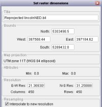Figure 3

Select the Edit->Edit raster menu item and click the Edit button in the Map Projection section.
Set the projection information to Latitude/longitude from the drop-down menu, and the ellipsoid to WGS84. Press the OK buttons in the projection and edit windows to confirm your selections.
Select the Transform->Reproject... menu item and in the window that appears, select UTM as the New Projection. This will produce a new window allowing you to set the dimensions of the new projected raster (see Figure 3)
In the new window, enter 30 in both the E-W Res and N-S Res fields. All the remaining fields can be left with their default values.
Click the OK button to create the reprojected raster.

After a few seconds, a new surface should appear as shown in Figure 4. Note that the index area now shows two images - the original as well as the reprojected surfaces. You can select any of the index objects at any time by clicking on the chosen image with the left mouse button. The more rectangular shaped surface now has a fixed resolution where each DEM cell represents a square of 30m x 30m on the ground.

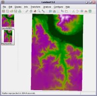Figure 4

Remove the original unprojected (square) DEM by clicking on its small index image with the left most button and then selecting Edit->Delete Raster. Once deleted, click on the reprojected raster in order to select it.
Check that the resolution of the reprojected raster is indeed 30m in both an east-west and north-south direction by displaying the summary information as you did above. You should also confirm that the raster now has 321 columns and 469 rows.
We will use this new surface in later stages of this tutorial, so save it by selecting either the File->Save... menu or the button. Call the file lincolnNED30m.srf and save it somewhere where you can later open it.

Step 3 - Displaying the Surface.

The images we have seen so far that represent the surface are made by allocating a colour to each cell value in the raster model. So for example, all cells that represent an elevation of around 500m above sea level are coloured green and all those that are 800m above sea level are purple. LandSerf can use this same elevation information to model the amount of light or shade on each raster cell by calculating local slope direction and steepness. This can be combined with the colouring scheme you have already seen to produce a shaded relief map of the surface:

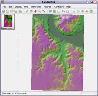Figure 5

To view a shaded relief representation select the Display->Relief menu item. This should produce an image similar to that shown in Figure 5.
Try altering the shaded relief parameters by selecting either the Configure->Shaded relief menu item or the button. In the new window that appears, you can move the sliders for each parameter and see the effect each has on the image. When you are happy with the parameter settings you have selected, press the OK button. After a second or two, the new shaded relief image should be displayed in the main window.

The colour scheme associated with any object can be changed, either by selecting one of LandSerf's pre-defined colour schemes, or by creating a series of colour rules to be associated with the object. At this stage, we will select one of the pre-defined colour schemes:

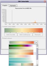Figure 6

Select the Edit->Edit raster menu option. This will display a window allowing you to alter many of the characteristics of the elevation surface.
Click the Edit button next to the colour bar about three quarters of the way down the window. This should display a colour editor window similar to that shown in Figure 6.
From the drop-down menu in the colour editor window, select the fourth colour scheme from the list (green to orange scheme).
You can refine the selected colour table by dragging any of the black vertical lines below the colour bar in the centre of the window. Each one of these lines represents a single colour and by dragging it to the left or right, you are attaching that colour to a given elevation value. You can also use the frequency histogram at the top of the window to see how many raster values will be associated with each colour.
When you are happy with the colour scheme you have created, press the OK button on the colour editor window and then the Edit Raster window.

You should now have a new shaded relief representation of the Lincoln elevation model shown in the main display area. LandSerf has used the key colours you have selected and interpolated new colour combinations between each of them to produce the continuously varying colours you now see.

You will notice that the northern part of our DEM is dominated by part of a large meandering river (the Columbia River) that is coloured green similar to the banks on either side. In order to distinguish the river from its surroundings, we can associate a unique colour with it by finding its elevation and attaching a discrete colour rule to that elevation alone:

Figure 7

New colour scheme with unique river colour

Figure 8

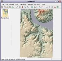To find out at what elevation the Columbia River lies within our model, we can put LandSerf into query mode by selecting either the Info->query map menu item or by pressing the button.
Once in query mode, try moving the mouse over the DEM representation. You should see the geographic position and elevation of the current mouse location being reported at the bottom of the window. Make sure you move the mouse over the river area and note its elevation (see Figure 7).
To move out of query mode, simply select the same option again which will toggle LandSerf back into its normal mode.
Bring up the colour editor window just as you did previously. This time, select the Numeric tab at the top of the window. This will display the colour scheme as a series of numeric rules rather than the graphical display we have previously seen.
To associate the elevation of the river we have just found out (394m above sea level) with a blue colour, type the following four numbers in the Edit colour rule field: 394 141 141 166. and then press the Add Discrete button. This will associate the red-green-blue colour combination represented by the triplet (141,141,166) with any raster cells with the value 394.
Finally, accept the changes you have made to the colour scheme by pressing the OK buttons in both the colour editor window and the raster edit window. You should now be presented with an image of the Lincoln DEM similar to that shown in Figure 8.

Sometimes the level of detail represented by an elevation model is greater than that displayed on the screen. It is therefore useful to be able to 'zoom in' to an image in order to examine it in greater detail. This is one way of exploring how the characteristics of a surface vary with scale.

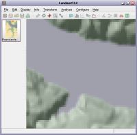A zoomed in portion of the DEM with new colour scheme

Figure 9

Put LandSerf into zoom mode by selecting either the Display->zoom mode menu item or by pressing the button.
Holding the left mouse button down, try moving the mouse up and down over the main image in LandSerf. This should allow you to zoom in and out of the map, centred on the location at which you first press the mouse down.
Holding the right mouse button down (or ctrl and mouse button on MacOSX), try moving the mouse up, down, left and right over the main image. This should allow you to 'pan' across the map. In combination with the zooming function, you should now be able to centre the map on any location of interest at any scale you wish.
Use the zooming and panning features to centre the map on the tributary identified in Figure 9.
To come out of zoom mode, simply press the zoom button or Display->zoom mode item again. You can restore the image to its original position and scale by selecting either the Display->Full image menu item, or the button.
Finally, save the surface with its new colour scheme just as you did at the end of Step 2.

Step 4 - Attaching metadata to Rasters.

A spatial object in LandSerf consists of the data (elevation values in the DEM we have used so far) and a collection of metadata attached to that object. We have already seen some of those metadata in the form of the georeferencing of the boundaries of the surface, the map projection used, the resolution of each raster cell and the colour rules used to display the raster. We can also create and examine other metadata such as the title, lineage and attribute categories associated with a spatial object.

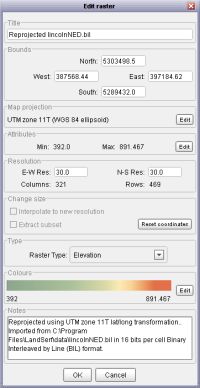Editable metadata associated with a raster

Figure 10

If you haven't just moved on from the previous step, load a saved copy of lincolnNED30m.srf into LandSerf.
Bring up the editable metadata by selecting the Edit->Edit raster menu option. This should display a window similar to Figure 10.
The title of the raster was created automatically when we previously projected it into UTM coordinates. Change it to something more explanatory by typing Lincoln 30m DEM in the Title field.
The 'Notes' field at the bottom of the window contains details of the original file used to create the raster as well as the UTM projection information. This information may be useful if we later wish to trace the lineage of the data. We can however add some further useful information about the source of the data. Add the following text to the bottom of the Notes field: Elevation data from USGS National Elevation Dataset (NED) available from http://seamless.usgs.gov
Accept these amendments to the raster by pressing the OK button, and save a copy of this object using either the File->Save... menu or the button.

LandSerf allows several datasets to be stored and displayed simultaneously. We will add a further raster layer representing landcover measured and classified from satellite remote sensing. We will then add some additional metadata to this new layer. Unlike elevation, landcover classes are categorical rather than direct measurements. Each cell is allocated a numeric value that represents a class of landcover (water, shrubland, woodland etc.). The value of that number is not directly important other than providing a unique identifier to a given landcover type.

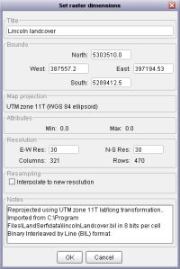Figure 11

Load the file lincolnLandcover.bil that is in ArcGIS Binary Image Layer (BIL) format and is stored in the data sub-directory of LandSerf (see Step 1 if you have forgotten how to do this).
These data are again georeferenced using latitude/longitude angles and therefore should be reprojected into UTM coordinates. As you did in Step 2, edit the raster information setting the projection type to Latitude/longitude and the ellipsoid to WGS84. Reproject the raster to UTM by selecting Transform->Reproject and in the window that appears, set the N-S and E-W resolutions both to 30m as you did previously, but this time make sure the Interpolate to new resolution box is not selected. This is because we wish to create a reprojected raster that only contains the same category values as the original dataset and not create new interpolated categories.
Give the raster a new title by typing Lincoln landcover in the Title field (see Figure 11). Press the OK button to perform the transformation.

We will change 4 elements of the new landcover dataset - the attribute labels; the colour scheme; the type of raster; and the lineage notes of the layer. These changes will make it easier to process and interpret any analysis we apply to the data at a later stage.

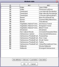Figure 12

Select the Edit->Edit raster to bring up the raster editor window.
The first element we will change will be the colours, so press the Edit button adjacent to the colour bar. This time, we select the colours from a colour table file, so press the Load colours button and select landcover.ctb and press the OK button to accept these colours (but leave the main Edit Raster window open). Note that because the landcover layer consists of categories, all the colour rules are discrete rather than the continuous rules we used for elevation.
Next we will associate labels with each of the categories of landcover. To do this press the Edit button of the Attributes area of the Edit Raster window. This should display a new Attribute Table window.
Press the Load table button and open the file landcover.atr. This file contains the labels associated with each of the numeric attribute values used by the raster. You should now have a table displayed similar to that shown in Figure 12. Click on one of the values in the third column to make these attributes 'active'. Finally press OK in this attribute window to accept the new table.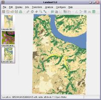

Figure 13

Before leaving the raster editor, we will change two more items of metadata. Firstly, you will notice that the Raster Type identified in the Type are of the window is set to Elevation. Select the drop-down menu in this area and change it to Other. This will prevent LandSerf from attempting to perform elevation-specific operations on the raster.
Finally, we will add some lineage information to the raster. Copy and paste the following into the Notes field of the editor window:
Originator: U.S. Geological Survey (USGS) Publication_Date: 19990631 Title: Washington Land Cover Data Set Edition: 1 Geospatial_Data_Presentation_Form: raster digital data Publication_Information: Publication_Place: Sioux Falls, SD USA Publisher: U.S. Geological Survey Online_Linkage: http://landcover.usgs.gov.
Save a copy of this newly amended raster as lincolnLandcover.srf.
We can query the new raster by putting LandSerf into query mode (see Step 3 above). As you move the mouse over the raster, the numeric and 'active' text labels associated with each cell in the landcover raster should now be displayed (see Figure 13).

Step 5 - Simple morphometric analysis.

We have already gained some impression of the landscape represented by our DEM simply by visualising it. We can assume for example that the landscape contains a large meandering river, some apparently mountainous region to the north, several tributaries flowing from the south of the DEM northwards into the river. We might characterise the region as a whole as 'hilly'. We also know from the landcover information that large parts of the landscape are grassland with some patches of woodland and agriculture.

Such description however has obvious limitations. It is subjective (you may have gained a different impression of the same landscape), it is rather vague (what exactly does 'hilly' mean?), and might simply be incorrect (are we sure that is a mountain to the north of the river or is it just a small undulation?). We can use LandSerf to provide us with a more systematic and objective description of the landscape; one that we can use to compare with other landscapes described by other people.

Firstly it is useful to make sure we have a good idea of the scale and extent of the landscape. We can do this by viewing the metadata associated with the DEM.

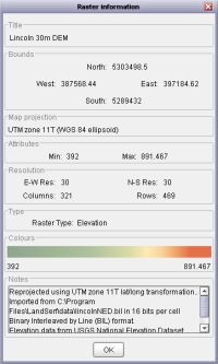Figure 14

If you haven't just moved on from the previous step, load a saved copy of lincolnNED30m.srf and lincolnLandcover.srf into LandSerf.
Make sure the Lincoln DEM is selected as the primary raster by clicking on its thumbnail view with the left mouse button.
Additionally we can select or deselect a secondary raster by clicking on one of the thumbnails with the right mouse button (or ctrl button press on MacOSX). Doing so will produce a grey border around the secondary raster while it is selected. Select Lincoln Landcover as the secondary raster and then and then Display->Relief. LandSerf should display a shaded relief map in the main area using elevation from the primary raster to calculate shading,and the thematic colours from the secondary raster to produce the colours of the map.
Try deselecting the secondary raster by clicking on its thumbnail with the right mouse (ctrl mouse press on MacOSX) button and then redisplaying shaded relief. You should now have a display of the DEM relief without any landcover information.
View the DEM information by selecting Info->Summary Info or the button. You should see that the raster consists of 321 columns and 469 rows with a resolution of 30m per DEM cell. This means we are viewing a landscape that is approximately 10km by 14km in extent. We also know from the information that the range of heights within this region is approximately 392m to 891m - a vertical range of about 500m.
Click the OK button to close this information window.

This vertical range or relief we have identified from the raster information window only gives us a broad summary of how elevation changes over the surface. We can get a more detailed view by examining the frequency distribution of elevation values.

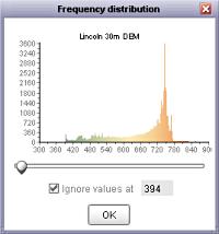Figure 15

Select either the Info->Histogram menu item or the button. This should display a frequency histogram in a new window.
You should notice that by far the most frequently occurring elevation value is at 394m, which corresponds to the height of the river Columbia. You can force the histogram to ignore values at this elevation by clicking the Ignore values at box and typing 394 in the text area to the right (see Figure 15).
You can change the category widths of the histogram by moving the slider left and right. The most obvious feature of the distribution is the peak in the histogram at about 750m. This corresponds to the plateau area that dominates the southern half of the DEM.
Close the histogram window by pressing the OK button.

So can we get a better idea of the 'roughness' of the terrain? One way of doing this is to measure the steepest slope at all cells in the DEM and visualise the results:

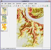Figure 16

Select either the Analyse->Surface Parameter menu item or the button. Select Slope from the list of properties and press the OK button. You should see a message Calculating Surface Parameterisation... appear at the bottom of the LandSerf window and a percentage progress indicated in the bottom-right corner. After a few seconds a new slope image should be displayed (see Figure 16). Slope is coloured from white (horizontal) through yellow to red (steepest slope). This new image shows the flat plateau in the south-west and the steeper slopes bordering the Columbia river and its larger tributaries.
We can examine the slope map in more detail by selecting it as the primary raster. Do this by clicking on the slope map thumbnail image with the left mouse button, and then Display->Raster to redisplay the slope map.
Try using the query mode and zoom mode to explore the slope map in more detail (see Step 3 if you have forgotten how to do this).
Display the frequency histogram of slope map (Info->Histogram or ). You may wish to widen the graph window so that the histogram bars are more obvious. The histogram is dominated by the large number of horizontal cells (corresponding to the plateau and the river surface) with steeper cells being relatively less common. This distribution shows an approximately log-normal distribution typically exhibited by many slope maps.
Save a copy of this slope map as lincolnSlope.srf for later analysis.

Slope represents one of the four surface parameters that are often used to characterise surface behaviour. The other three are aspect which identifies the azimuthal direction of steepest slope, profile curvature, which describes the rate of change of slope in profile, and plan curvature, which describes the rate of change of aspect in plan. We shall use LandSerf to view each of these in turn:

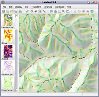Figure 17

Make sure the Lincoln DEM is selected as the primary raster by left-clicking its thumbnail view. Set the display to show shaded relief.
Select Analyse->Surface Parameter (or the button), but this time choose Aspect from the list of properties and press the OK button.
Use the techniques you have used so far, such as zooming, querying and histogram calculation to identify any further characteristics of the DEM. Repeat this task for Profile Curvature and Plan Curvature (see Figure 17) measures.

Finally, we shall examine one further characterisation of the surface. Rather than measure surface parameters we can classify the terrain into surface features using some of the parameters we have already investigated. One of the commonest (and most useful) classifications is to group all points on a terrain into one of the following:

pits
channels
passes
ridges
peaks
planar regions

This can be done by measuring both the slope and curvature of each cell in the DEM and performing the appropriate classification (for more details on how this may be done see the theory documentation). We will perform such a classification on our DEM:

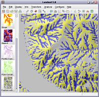Zoomed in portion of the feature classification map

Figure 18

Make sure the Lincoln DEM is selected as the primary raster by left-clicking its thumbnail view. Set the display to show shaded relief.
Select Analyse->Surface Parameter (or the button), and choose Feature extraction from the list of properties and press the OK button.
You should see a predominantly grey, blue and yellow image appear. The grey areas represent planar regions, blue areas represent channels and yellow ridges. If you look carefully (you may have to use the zoom mode to see this), you should also see occasional red cells that represent local peaks and green cells that represent passes in the landscape (see Figure 18).
Save a copy of this feature classification by selecting it as the primary raster (left-click its thumbnail image) and saving it with the name LincolnFeatures.srf.

Feature classifications like this are useful for several reasons. The pattern of channels appears somewhat similar to a drainage network, thus giving us an idea of where water would flow over the surface. Perhaps less obviously the pattern of yellow cells gives us an equivalent ridge network, identifying portions of the landscape where water is likely to flow from. Consequently, the ridge network is related to the drainage divides/watersheds that define drainage basins. In theory at least, the green passes identify points of intersection between the channel and ridge networks. Along with pits and peaks, passes represent what are sometimes called surface specific points - points on the landscape that carry special significance in its structure.

Step 6 - Advanced morphometric analysis.

When we wish to characterise a real terrain using a computer, the closest we can get is to characterise the elevation model that represents it. In doing so we hope that the model is sufficiently accurate for the purposes of analysis. As far as possible we should strive to produce characterisations of landscape that are as dependent as possible on the surface we are interested in, but as independent as possible of the particular model we have used.

One of the most significant limitations of the models and processing we have carried out so far has been the scale of analysis implied by the DEM resolution. You will remember that each cell in the Lincoln DEM is 30m x 30m. Since most of the analytical functions we have used so far work by comparing one cell with its 8 adjacent neighbours, the results of that analysis are likely to be at the resolution of approximately 3 times the grid cell size. So for example, the blue valleys we identified in the previous step will be those that have a width around 30-90m. This scale is really rather arbitrary; we might be more interested in characterisation of features have expression over 1km or 10cm. Unfortunately, the DEM cannot provide us with direct information at a finer scale than its resolution (30m), but we can use it to perform analysis at a broader scale.

The basis for most of the analytical functions in LandSerf is the process of quadratic approximation (see theoretical details on surface characterisation for further information). This involves taking a local window of DEM cells (3 x 3 in the examples we have seen so far), and fitting the most appropriate continuous quadratic function through them. LandSerf then uses this quadratic function to calculate parameters such as slope and curvature. We can set the size of the local window that LandSerf uses before it does any calculation. This allows us to perform analysis at much broader scales than that implied by the DEM resolution.

Firstly, we will view the effect of changing window size by smoothing out features that are smaller than about 330m wide. Since each cell is 30m, we will need to process the surface using window sizes of 11x11 cells rather than 3x3:

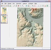Figure 19

If you have just moved on from the previous step, delete all rasters except the Lincoln DEM. To remove an object from LandSerf, select it as the primary raster with the left mouse button, then select the Edit->Delete raster menu option.
Make sure the Lincoln DEM is the primary raster and that display is set to Shaded Relief.
Select either the Configure->Window scale... menu item or the button, and set the window size to 11 rather than 3 (we shall leave the 'distance decay exponent' set to 0). Press the OK button to close the dialogue box.
By changing window scale, any subsequent analysis will be performed at this new 330m scale. To demonstrate this effect we shall reinterpolate our DEM at the new scale. Select Analyse->Calculate Surface Parameter (or the button) and choose the Elevation item. You will notice that processing at this new scale takes longer than previous examples since LandSerf is having to process 13 times as many cells for each calculation.
To view the effect of this smoothing, select the Smoothed Elevation layer as the primary raster and then Display->Refresh (see Figure 19). You can quickly alternate between the original and smoothed DEM by selecting either as the primary raster and then pressing Ctrl-R to refresh the display.

The result of broadening the scale of analysis is to smooth out many of the finest scale details while leaving the larger features of the landscape unaltered. You may also notice that the entire raster also appears smaller than the original. This is produced because analysis based on square windows of size nx n cannot process cells within (n-1)/2 cells of the edge. As a consequence, LandSerf fills the border cells of the raster with null values that are not displayed or processed.

We can see the effect of further broadening the scale of analysis by setting the window size to 65 (corresponding to a distance on the ground of 65*30m = 1.95km):

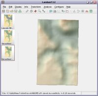Figure 20

Make the original DEM the primary raster and then set the window size to 65 ( Configure->Window scale... or ).
Select the Analyse->Calculate Surface Parameter menu item, and choose the Elevation option again. Processing will be much slower this time as LandSerf is now processing 470 times as many cells as the original 3x3 window. This might be a good time to make yourself a cup of coffee. If you ever find yourself waiting for a very slow process to complete in LandSerf, you can always stop it by clicking somewhere on the process bar in the bottom-right corner.
When you have drunk your cup of coffee and LandSerf has finished calculating the surface, view it by making it the primary raster and refreshing the display.
Save a copy of this smoothed DEM as lincolnNED65.srf for later use.

So do the parameters that we can measure from the surface also vary if we calculate them at this new broader scale? We can find out the answer to this question by measuring a surface parameter at many different scales and seeing how it varies:

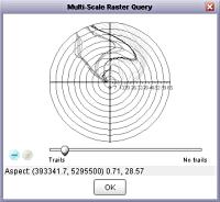Figure 21

Make the original unsmoothed DEM the primary raster and ensure the display is refreshed.
Select Info->Multiscale query... and choose Aspect as the surface parameter to examine. Press the OK button to display the multi-scale query window (see Figure 21).
Move the new window so it is not overlapped by the main LandSerf window and resize it if it is too small. Try clicking the mouse at various point on the main DEM display. The query window shows how aspect varies with scale. The line drawn on the graph shows the direction of steepest slope measured from 3 x 3 windows at the centre to 65 x 65 cell windows at the outer edge. If the line remains in a relatively constant direction, aspect is said to be scale-invariant at this location. If the line appears to meander as it moves out from the centre, the slope direction must be dependent on the scale at which it is measured. A numerical measure of this dependency is shown in the bottom of the window. The first two numbers give the location of the point being queried, while the second two give the (circular) mean and standard deviation of the aspect measure.
If you try dragging the mouse over the DEM, the aspect graph is updated continuously. This allows you to investigate the spatial pattern of scale dependency. By moving the 'trails' slider to the left or right, you can control how much of a 'query history' is displayed on the graph. This allows you to explore visually, the spatial variation in scale dependency.
By dragging the mouse over the main DEM display, identify which parts of the landscape produce scale-invariant measures, and which produce scale-dependent measures. Are there any critical scales at which aspect does not vary over space?

We will use a similar process to explore the scale dependency of other measures.

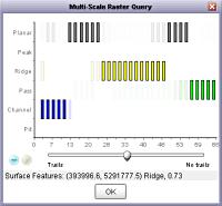Multiscale query of feature classification

Figure 22

Leaving the aspect query window open reselect the Info->Multi-scale query... menu item. Choose Profile curvature and click or drag various points on the DEM. The maximum size of the query window (representing processing of a 65x65 cell window in this case) is indicated by the black square on the main display. Try to relate the curve plotted and the location and character of the landscape you have queried.
Repeat this step with some of the other measures, including feature classification (see Figure 22) in order to investigate the degree to which their measurement is dependent on the scale of analysis.
When you have finished, close all the query windows by clicking their OK buttons.

One of the advantages of multi-scale processing of terrain is that we can relate our analysis to scales that are of most interest to us. We shall round of this section by calculating the network of surface features at two different scales. First we shall identify the network of ridges and channels at a fine scale:

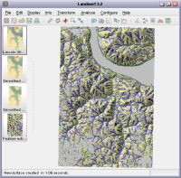Figure 23

Making sure the Lincoln 30m DEM is selected as the primary raster, select Configure->Window scale... (or ) and set the window size to 5 and the distance decay exponent to 1.0. This will set the processing back to using a 5 x 5 cell window, but additionally, by specifying a positive distance decay value, we have told LandSerf to give a greater weighting to cells nearer the centre of a window than ones that are further away. The higher the value of this exponent, the greater the importance given to near cells in the calculation of parameters such as slope and aspect.
Select Analyse->Calculate Surface Parameter (or ) and this time choose the Feature network extraction option. This will will produce a similar classification to the surface features seen previously, but will emphasise the network of channels and ridges (see www.soi.city.ac.uk/~jwo/sdh98 for more details of this process). Even so, you should see that the resultant image is still somewhat discontinuous - both the blue channel network and the yellow ridge network have plenty of gaps.

We can improve the representation of the network by forcing LandSerf to connect some of these ridges and channels together. As this network would describe the topology of the surface, LandSerf will represent it using a vector rather than raster coverage:

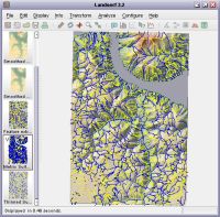Figure 24

Select either the Analyse->Vector Feature Network menu item or the button. This will process the raster network and after a minute or so, will produce a vector network and new thinned raster version of the network.
To display the vector over the original DEM, unselect the thinned raster network as the secondary raster by right-clicking (ctrl-clicking on MacOSX) on its thumbnail view. Select the Display->Vector to see the metric surface network (see Figure 24). You may wish to use the zoom mode to examine the network in greater detail.
For more details on Metric Surface Networks, see www.soi.city.ac.uk/~jwo/geoComp2000.

Notice how both the blue channel network and the yellow ridge network appear similarly tree-like. The plateau to the south-west is dominated by local passes, pits and peaks (green, black and red dots). This is because at this scale, errors in the DEM tend to dominate flatter regions. We can broaden our scale of analysis, and therefore reduce the impact of DEM error, by repeating the process using a larger window size:

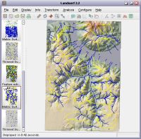Figure 25

Set the window size to 25 (corresponding to a distance of 25 x 30 = 750m on the ground) leaving the distance decay value at 1.0.
Select the Analyse->Calculate Surface Parameter menu item and again choose Feature Network Extraction and press the OK button.
Select Analyse->Create Vector Feature Network ( ) to start the network calculation.
When complete, you can again display the vector over the original DEM, by unselecting the new raster thinned network and refreshing the display (see Figure 25). You can contrast this broader scale network that represents the topology of larger ridges and channels with that of the finer scale network produced previously.
You may wish to save a copy of the vector network for later analysis. To do this select File->Save... () and then set the Files of type drop-down menu to LandSerf vector and save the file with the name LincolnMSN25.vec.

This ends the tutorial. This has been an introduction to LandSerf and the process of terrain analysis. To get the most of the software, you should experiment with some of the other functions available and apply them to your own data. See the user guide for more details.