A Brief Introduction to Python

Aidan Slingsby a.slingsby@city.ac.uk

This introduction is intended for those who already have some familiarity with python. You should know what variables, functions, operators are and how loops and if statement work. The most important thing you can do is practice. This tutorial won't give you much practice. But it will help to show how Python fits together, some general principles, and how we will be using it during the MSc in Data Science. We will make reference to the W3 Schools' Python tutorial which gives the basics.

Please install Anaconda and check that the Spyder editor works, in advance. Anaconda is a suite of Python tools that includes Python itself. See below for more details.

Introducing Python

Python is an interpreted, high-level, general-purpose programming language that works on many platforms. Its popularity for Data Science is largely down to its simplicity and the huge number of libraries that are available for it. There are a only few basics to learn, but note that most of your work will be using libraries and most of your Python effort will be about learning how to use individual libraries.

It is relately easy to write Python by hacking together code from examples on the web, but I recommend that you try and understand the syntax and how this code works. This will make things easier in the long term.

Python has been around since the early 1990s, but 2008 saw the release of Python 3, a major revision that is not completely compatible with previous releases.

Before you start this, please install Anaconda on your computer (see below).

Anaconda

Python is free. We will be using the Anaconda distribution, which includes a suite of tools including those that help you install/update libraries. Install it here and see the quick instructions in their cheatsheet.

"Spyder" as a Python editor

Python code is simply plain text file. You can write it in any editor that saves plain-text (e.g. Notepad) and then running this file through a python interpreter to execute it (python myPythonCode.py).

However, using specific python editor makes life a bit easier for us. We will be using the "Spyder" editor in this tutorial, because it contains a lot of built-in tools for helping you write python. It is part of Anaconda, so you will have it on your computer. Other editors will be covered later. You can launch it from the Anaconda Navigator.

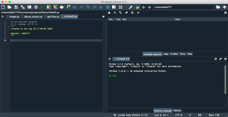
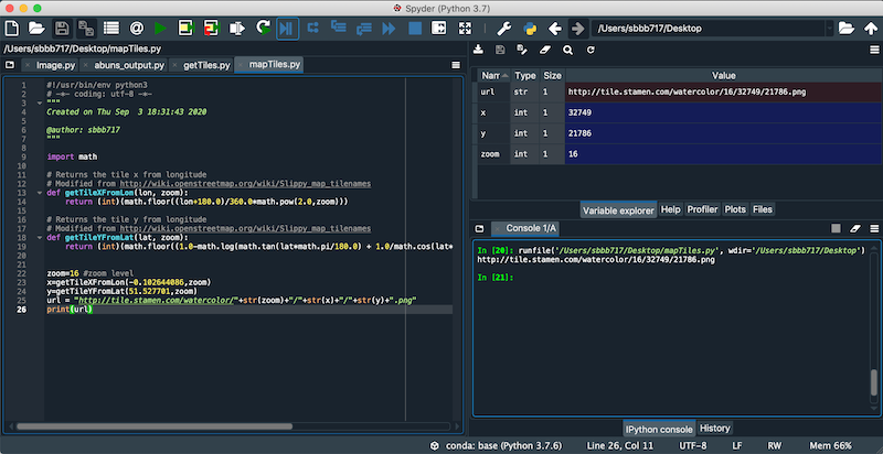
I want to draw your attention to three panels of the Spyder interface:

• Code (left): this is where your python files can be edited
• IPython console (bottom right): to run python commands immediately
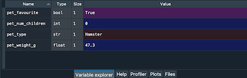
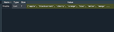
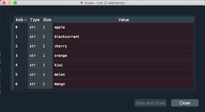
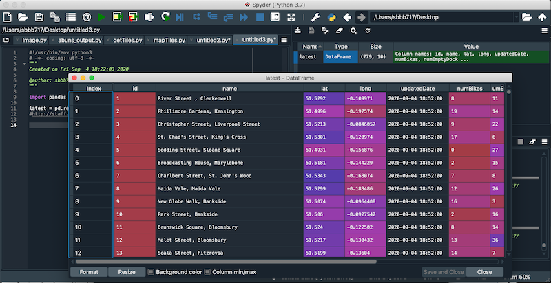
• Variable explorer (top right): to see what variables you have

Write your first line of python in the traditional way by pasting the following into the IPython console:

print("Hello world")

Hello world

Syntax and comments

See the basic syntax and comments. Unlike most languages, indentation has meaning (that we'll come on to) so don't accidentally give your code different indentation.

Variables

Variables are named labels that represent values or more complex types of data. Don't make life difficult by using uninformative variable names such as my_number - try and make your code understandable.

In python, conventionally, variables start with a lowercase letter and use the _ character to separate words. Variables names cannot start with numbers, cannot contain spaces, can only have alphanumeric characters of _, and are case-sensitive.

There's no need to declare them in advance, you just initiate them using the = assignment operator. If it already has a value, it will be overwritten.

Once a variable is initialised, we can easily access the value (and change it if we like). Note that variables persist, so unless you go to the Consoles menu item and select Remove all variables they'll all still be there.

Type the following into the IPython console in Spyder:

pet_type = "Hamster"
pet_weight_g = 47.3
pet_favourite = True
pet_num_children = 0

Print the values to screen:

print(pet_type, pet_weight_g, pet_favourite, pet_num_children)

Hamster 47.3 True 0

Now take a look at the "variable explorer".

The four variables are listed along with their (inferred) types and their values. This is one of the advantages of using a python editor.

You can also see what types of variables are, by using the built-in type() function (also using the built-in function print():

print(type(pet_type))
print(type(pet_weight_g))
print(type(pet_favourite))
print(type(pet_num_children))

<class 'str'>
<class 'float'>
<class 'bool'>
<class 'int'>

Data types

As you've seen, variables can be of different data types.

Data types that store single values

bool is for a True/False Boolean value which can also be represented as 0 or 1.

int and float are for whole and non-whole numbers respectively.

str is for text. If you specify text directly in Python, it needs either single or double quotes around it.

Data types that are collections that store more than one value

A list is a collection of values that is ordered (i.e. a sequence) and for which you can change the values. Values can be any data type (even lists!) but normally they'd be of the same type. Square brackets are used to create, access and change values in lists. List indexes start from zero, so fruits[1] is the second item.

#Create a list of `str` values (using single or double quotes)
fruits = ["apple", "banana", "cherry", "orange", "kiwi", "melon", "mango"]

print(fruits)        
print(type(fruits))       #to how that this variable is a list
print(fruits[1])          #to show the SECOND item in the list
print(type(fruits[1]))    #to show that the item is a str
print(fruits[-1])         #negative values are from the end of the list (last value)
print(fruits[2:5])        #a range
print(type(fruits[2:5]))  #to show this is a list
print(fruits[:4])         #from the first item to the fifth
print(fruits[2:])         #from the the third item to the end
fruits[1] = "blackcurrant"#change the second item in the list
print(fruits)

['apple', 'banana', 'cherry', 'orange', 'kiwi', 'melon', 'mango']
<class 'list'>
banana
<class 'str'>
mango
['cherry', 'orange', 'kiwi']
<class 'list'>
['apple', 'banana', 'cherry', 'orange']
['cherry', 'orange', 'kiwi', 'melon', 'mango']
['apple', 'blackcurrant', 'cherry', 'orange', 'kiwi', 'melon', 'mango']

You can also see these in the variable explorer (click the list to get the table)

The str type is actually a list of characters, so individual letter and substrings can be accessed from strings using the techniques above.

message = "Unhappy!"
print(message[2:])

happy!

A set is like a list, but unordered and cannot have duplicates. It is created using curly brackets. Since it's unordered, you can't access individual elements except by looping through the list (see later).

A dictionary (dict) is really useful. It stores key-value pairs allowing you to relate information. Keys are unique, but you can have as many values as you want. Continuing the fruits example, we could store the colour of each fruit. In this example, both the keys and values are str data types.

#Create a dictionary of `str` values (using single or double quotes)
fruit_colours = {"apple":"green/red", "banana":"yellow", "cherry":"red", "orange":"orange", "kiwi":"green", "melon":"yellow", "mango":"orange"}
print(fruit_colours)

print("A banana is",fruit_colours['banana']) #access the value with the key "banana"

{'apple': 'green/red', 'banana': 'yellow', 'cherry': 'red', 'orange': 'orange', 'kiwi': 'green', 'melon': 'yellow', 'mango': 'orange'}
A banana is yellow

Dictionaries are used extensively when doing data science with Python. Values can be of any data type. Examples of their use are:

• substituting values e.g. replacing country codes with names (see [example])(https://stackoverflow.com/questions/12906090/country-name-from-iso-short-code-in-dictionary-how-to-deal-with-non-ascii-chars)
• mapping colours to values in charting libraries
• setting parameters in some python libraries

A tuple is like a list, but values can't be changed (immutable). Generally its used differently to lists - to store a set of values what describe something (like a coordinate). Often returned by functions, they use round brackets (( and )) in their construction.

Data types that are classes

We'll come onto classes later. In actual Python is an object-oriented language and all data types are classes and values are objects (or class instances). We'll look later at how classes can:

• represent complex data types comprising a mixture of different data types
• have their own functions that operate on the objects themselves

Most Python libraries use classes to implement sophisticated and complex behaviour as we'll see.

Typecasting

When we type data values into our code, Python guesses the data type. We can also cast the data type by telling Python to treat it like another data type. We do this by using the type name like a function.

pet_weight_g = 47          #will be inferred to be an int
print(type(pet_weight_g))
pet_weight_g = float(47)   #specify to treat as a float
print(type(pet_weight_g))

<class 'int'>
<class 'float'>

Operators

Operators operate on data. The ones you'll use most are arithmetic operators, assignment operators, comparison operators and logical operators, but there are also identity operators, membership operators and bitwise operators.

Some operators work differently depending on the data types. + is arithmetic addition if the values are numerical; but it joins (concatenates) values together if the values are str types.

Loops

For loops let you repeat things, either a fixed number of times or iterate through a list. Indentation is essential.

#Fixed number of times
for i in range(6):
  print(i)

0
1
2
3
4
5

#Iterate over a collection
fruits = ["apple", "banana", "cherry", "orange", "kiwi", "melon", "mango"]
for fruit in fruits:  #iterates through all the fruits
  print(fruit)

apple
banana
cherry
orange
kiwi
melon
mango

There are also while loops.

If statements

If statements work in the same way as in many languages, and require the use of operators, and use indenting.

#Print only odd numbers (% operator here is modulus, if you divide a (whole)
#odd number by 2, you'll get 1)
limit=10
print("Odd numbers from 0 to",limit)
for i in range(limit):
    if i%2==1:
      print(i)

Odd numbers from 0 to 10
1
3
5
7
9

Functions

A function (usually) names a block of code which only runs when it is called. You can pass it arguments (args; of various data types) and it can return values (of various data types).

So far, we've been using Python's built-in functions such as print() and type(). Functions may take any number of parameters (including none) of different types and may return any number of values of different types.

Programming by example is great, but it's worth learning to read documentation. The good news is that it's really easy to get a summary of how a method works: In a Jupyter notebook, you can just put a ? followed by the function name e.g. ? print. In the Spyder console you can either type the function e.g. print() and a pop up will provide summary information or you can achieve the same result by using the help function e.g. help(print)

? print

Docstring:
print(value, ..., sep=' ', end='\n', file=sys.stdout, flush=False)

Prints the values to a stream, or to sys.stdout by default.
Optional keyword arguments:
file:  a file-like object (stream); defaults to the current sys.stdout.
sep:   string inserted between values, default a space.
end:   string appended after the last value, default a newline.
flush: whether to forcibly flush the stream.
Type:      builtin_function_or_method

The bad news is that this documentation is inconsistent and can be rather cryptic. It will help you to learn how to interpret them, which you may have to do in conjunction with a bit of Googling to find the web documentation. Hopefully this will prompt you to write good documentation!

The print function

What this (above) means is:

• "prints the values to a stream, or to sys.stdout by default"
• it takes *any number( (denoted by ...) of arguments called `value'
• an (optional) keyword argument (kwarg) called sep with a default value of (a space)
• an (optional) keyword argument (kwarg) called end with a default value of \n (a new line)
• an (optional) keyword argument (kwarg) called file with a default value of sys.stdout (standard output is usually the screen)
• an optional keyword argument (kwarg) called flush with a default value of False

The keyword parameters (kwargs) are optional. An example of the used of 'sep' is thus:

pet_type = "Hamster"
pet_weight_g = 47.3
pet_favourite = True
pet_num_children = 0

print(pet_type, pet_weight_g, pet_favourite, pet_num_children, sep=" - ")

Hamster - 47.3 - True - 0

Note that this extra optional named argument simply changes the separator when writing out these values.

The type function

? type

Init signature:  type(self, /, *args, **kwargs)
Docstring:     
type(object_or_name, bases, dict)
type(object) -> the object's type
type(name, bases, dict) -> a new type
Type:           type
Subclasses:     ABCMeta, EnumMeta, NamedTupleMeta, _TypedDictMeta, _ABC, MetaHasDescriptors, _TemplateMetaclass, PyCStructType, UnionType, PyCPointerType, ...

The type() method actually has some different variants. Ignore all, but the one we've been using: the middle one (after the Docstring: line):

type(object) -> the object's type

This:

• takes a parameter called object (which can be any variable for any type/object)
• return the type

So this method return a type object, as illustrated. The print() method prints class XXX where XXX is the data type.

pet_type = "Hamster"
print(type(pet_type))         #returns a string
print(type(type(pet_type)))   #return an object of class `type`

<class 'str'>
<class 'type'>

The pow function

Finally, let's look at pow, one of the built-in arithmetic functions.

? pow

Signature:  pow(base, exp, mod=None)
Docstring:
Equivalent to base**exp with 2 arguments or base**exp % mod with 3 arguments

Some types, such as ints, are able to use a more efficient algorithm when
invoked using the three argument form.
Type:      builtin_function_or_method

This raises x to the power of y, with an options kwarg z which is None by default. This is clearer in the web documentation. This:

• take two arguments, x and y (with an optional z)
• returns the answer

It also notes that the ** operator does the same thing.

Using methods from other modules and packages

A module is simply a python file that has a set of functions and/or constants (like variables, but cannot be changed) defined. Modules may be organised into packages. Python has a lot of prefined modules that give you amazing functionality. You use them, you simply import them, like:

import math

You can see what's available within a module (note that those that start with __ are generally internal ones that we wouldn't normally call). You'll also find the documentation on the web

dir(math)

['__doc__',
 '__file__',
 '__loader__',
 '__name__',
 '__package__',
 '__spec__',
 'acos',
 'acosh',
 'asin',
 'asinh',
 'atan',
 'atan2',
 'atanh',
 'ceil',
 'comb',
 'copysign',
 'cos',
 'cosh',
 'degrees',
 'dist',
 'e',
 'erf',
 'erfc',
 'exp',
 'expm1',
 'fabs',
 'factorial',
 'floor',
 'fmod',
 'frexp',
 'fsum',
 'gamma',
 'gcd',
 'hypot',
 'inf',
 'isclose',
 'isfinite',
 'isinf',
 'isnan',
 'isqrt',
 'ldexp',
 'lgamma',
 'log',
 'log10',
 'log1p',
 'log2',
 'modf',
 'nan',
 'perm',
 'pi',
 'pow',
 'prod',
 'radians',
 'remainder',
 'sin',
 'sinh',
 'sqrt',
 'tan',
 'tanh',
 'tau',
 'trunc']

An example is the math module. See the documentation here and you can use them like this:

print("PI is ", math.pi)

PI is  3.141592653589793

Making your own functions.

Making your own function is worth doing if there's some simple functionality that's small in scope you want to reuse.

One example is to construct a URL to get some data based on some parameters.

Stamen are a design company (amongst other things) have designed some really nice maps that look like watercolour. These map tiles are on a tile server and they provide an API to grab those tiles - it's simply a URL as described on their website:

https://tiles.stadiamaps.com/tiles/stamen_watercolor/{z}/{x}/{y}@2x.jpg?api_key=6ace8e1f-ea73-40a9-898e-a6978a5d4b67

The OpenStreetMap website (on which Stamen maps are based) describes how to convert latitude and longitude into these x and y values, providing pseudocode.

n = 2 ^ zoom
xtile = n * ((lon_deg + 180) / 360)
ytile = n * (1 - (log(tan(lat_rad) + sec(lat_rad)) / π)) / 2

We can convert this to two Python functions (always reference any sources you use!)

import math

# Returns the tile x from longitude
# Modified from http://wiki.openstreetmap.org/wiki/Slippy_map_tilenames
def getTileXFromLon(lon, zoom):
    return (int)(math.floor((lon+180.0)/360.0*math.pow(2.0,zoom)))

# Returns the tile y from longitude
# Modified from http://wiki.openstreetmap.org/wiki/Slippy_map_tilenames
def getTileYFromLat(lat, zoom):
    return (int)(math.floor((1.0-math.log(math.tan(lat*math.pi/180.0) + 1.0/math.cos(lat*math.pi/180.0))/math.pi)/2.0 *math.pow(2.0,zoom)))

We need to use the math module, w Note that variables initialised in functions can only be seen within the function. Also note that the indenting is essential to define the function block.

We can then use them, just like any other function. Note here that I'm typecasting the numbers to strings (though this may not be necessary).

zoom=16 #zoom level
x=getTileXFromLon(-0.102644086,zoom)
y=getTileYFromLat(51.527701,zoom)
url = "https://tiles.stadiamaps.com/tiles/stamen_watercolor/"+str(zoom)+"/"+str(x)+"/"+str(y)+".jpg?api_key=6ace8e1f-ea73-40a9-898e-a6978a5d4b67"
print(url)

https://tiles.stadiamaps.com/tiles/stamen_watercolor/16/32749/21786.jpg?api_key=6ace8e1f-ea73-40a9-898e-a6978a5d4b67

Try putting this URL in your browser.

Try putting this code into its own method.

In actual fact, the OpenStreetMap website does provide a function:

import math
def deg2num(lat_deg, lon_deg, zoom):
  lat_rad = math.radians(lat_deg)
  n = 2.0 ** zoom
  xtile = int((lon_deg + 180.0) / 360.0 * n)
  ytile = int((1.0 - math.asinh(math.tan(lat_rad)) / math.pi) / 2.0 * n)
  return (xtile, ytile)

Note that this does this all in one method, returning the two values as a tuple. Again, note the indentation.

Document your functions

It's good practice to provide documentation so that someone else can type ? yourFunction and get a good summary.

The help for the function we wrote is

? getTileXFromLon

Signature:  getTileXFromLon(lon, zoom)
Docstring: <no docstring>
File:      /var/folders/qp/833_d7651js_jq_n0ydl3k480000gp/T/ipykernel_29853/830997071.py
Type:      function

Note the <no docstring>. Let's add one.

def getTileXFromLon(lon, zoom):
  """Finds the Staman tile x from the longitude
    Parameters:
    argument1 (lon): Longitude
    argument2 (zoom): Zoom level (int from 0-16)

    Returns:
    int: The tile's x
   """
  return (int)(math.floor((lon+180.0)/360.0*math.pow(2.0,zoom)))

?getTileXFromLon

Signature: getTileXFromLon(lon, zoom)
Docstring:
Finds the Staman tile x from the longitude
Parameters:
argument1 (lon): Longitude
argument2 (zoom): Zoom level (int from 0-16)

Returns:
int: The tile's x
File:      /var/folders/qp/833_d7651js_jq_n0ydl3k480000gp/T/ipykernel_29853/3365258485.py
Type:      function

That's better!

Using python source code files

So far, we've been putting python in the IPython console, where it runs immediately.

Let's instead write code in a file. In Spyder, Choose File > New file from the menu. This will create a new python file (extension .py) in some temporary location. You'll probably want to save it somewhere, perhaps call it mapTiles.py.

Put the functions we made and the code to generate the tile URL in there and then run is (green triangle. Note that in the IPython console, it issues the runFile() function to run your file. This is also where the output goes.

Note that the variables are accessible to both, because it's all run through the IPython console.

Autocomplete and documentation

Spyder also give you autocomplete and documentation. Press tab after typing the beginning of a function and will list the available functions, tell you what the arguments are and even give you the documentation.

Cells

Another structural thing is cells. #%% breaks your code into cells which can be run separately (using the button with green triangle with yellow square on). Note that this calls the runcell() function in the IPython console.

Keyboard shortcuts

Learn the keyboard shortcuts. Here are some.

Debugging

This incredibly powerful feature lets you pause the execution of code and show you how the code executes and what the variable values are at any point. Add one or more breakpoints by clicking to the right of the line number. Then if you run it using the "debug file" button or menu option, the code will pause at the breakpoint. The buttons to the right of the debug button will allow you to step through the code, including into functions that are called. Whilst execute is paused, you can see the current state of the variables.

Have a go at using this on a loop:

sum=0;
for i in range(6):
    sum+=i
print(sum)

15

Classes and objects

Python is an object-oriented language, in that everything is an object. Objects not only hold data, but they hold functions that manipulate those data. These are defined by its class; effectively a template for the object. And you can find out what functions a class has by using the dir() function.

dir(str)

['__add__',
 '__class__',
 '__contains__',
 '__delattr__',
 '__dir__',
 '__doc__',
 '__eq__',
 '__format__',
 '__ge__',
 '__getattribute__',
 '__getitem__',
 '__getnewargs__',
 '__gt__',
 '__hash__',
 '__init__',
 '__init_subclass__',
 '__iter__',
 '__le__',
 '__len__',
 '__lt__',
 '__mod__',
 '__mul__',
 '__ne__',
 '__new__',
 '__reduce__',
 '__reduce_ex__',
 '__repr__',
 '__rmod__',
 '__rmul__',
 '__setattr__',
 '__sizeof__',
 '__str__',
 '__subclasshook__',
 'capitalize',
 'casefold',
 'center',
 'count',
 'encode',
 'endswith',
 'expandtabs',
 'find',
 'format',
 'format_map',
 'index',
 'isalnum',
 'isalpha',
 'isascii',
 'isdecimal',
 'isdigit',
 'isidentifier',
 'islower',
 'isnumeric',
 'isprintable',
 'isspace',
 'istitle',
 'isupper',
 'join',
 'ljust',
 'lower',
 'lstrip',
 'maketrans',
 'partition',
 'replace',
 'rfind',
 'rindex',
 'rjust',
 'rpartition',
 'rsplit',
 'rstrip',
 'split',
 'splitlines',
 'startswith',
 'strip',
 'swapcase',
 'title',
 'translate',
 'upper',
 'zfill']

And for each method, we can use ?

? str.capitalize

Signature:  str.capitalize(self, /)
Docstring:
Return a capitalized version of the string.

More specifically, make the first character have upper case and the rest lower
case.
Type:      method_descriptor

As you know, str is a class. You can use these methods by using a . after the variable name. For example:

myName="aidan"
print(myName)
print(myName.capitalize())

aidan
Aidan

So what you been to know is that a class is a data type, and object is the value that contains variable and functions. So a str variable actually references a more complex object that you might have expected with the ability to do things. This is a fundamental characteristic of object oriented language.

In practice terms for Data Science is when we use libraries that do complicated machine-learning, the complexity is hidden inside the objects that we use. And we can query and manipulate these objects by using the documented functions.

If you have a look again at the Dictionary documentation, you'll notice reference to many functions that help use dictionaries. Yes, you've guessed it... dictionaries are actually classes and have built-in functions that relate to use of dictionarys.

Defining your own class

Just like functions you can define your own bespoke classes to package together related data and associated functions for that data.

Below we can see a simple example of a class.

For the most part you will not need to define your own classes but it is useful to see how classes are defined in Python as it will allow you to understand how to interact and work with other classes built by others (eg. builtin classes and impprrted libraries (see next section))

class Person:
    """This defines an object of type Person that has a name and age attribute.
    The Person class will return a statement describing who they are and what age they are"""
    def __init__(self, name, age):
        self.name = name
        self.age = age
    
    def myname(self):
        print("Hello my name is " + self.name)
        
    #def myage(self, ):TO DO!
        

p1 = Person("John", 36)
p1.myname()

p2 = Person("Gina", 56)
p2.myname()

Hello my name is John
Hello my name is Gina

The class object is defined using the argument class followed by the name of the class. You can define your class by any name.

Most classes will have a __init__ method which is where you can initialise your class with any number of attributes so here we are providing the class object with name and age attributes.

The arguments that are provided to the __init__ method indicate what arguments we need to provide to the class when we call the class. So when we first define (or instantiate) class, we provide it with those required arguments:

p1 = Person("John", 36)

Now p1 defined here is an example or an "instance" of our Person class and we can define any number of Person class instances eg.

p2 = Person("Gina", 56)

Within the class we can define specific methods that are associated with processesing the data packaged within the Person class. So myname is a method that will take the name attribute and print a statement describing the name of a particular person class instance.

eg. p1.myname()

Returns: Hello my name is John

The first argument in each of these methods contains this argument self. This argument indicates that in order to call this function we must first instantiate the class in other words we must first define the variable p1 before we can call the method myname().

Now over to you to have a go at defining a myage method that will print out a statement describing the age of the specific class instance.

Libraries

Now we'll talk about libraries. Libraries are "packages" (collections of modules) that define classes and functions for some specific functionality. This is what makes Python (and other languages so powerful).

Example: Which bike hire station in London currently holds the most bikes?

This example will tell ous which bike hire station in London has the most bikes available.

The data is provided by Transport for London as an XML file - https://tfl.gov.uk/tfl/syndication/feeds/cycle-hire/livecyclehireupdates.xml. Try it in a browser! It's live (used by apps that tell you how many bikes there are at stations. Some browsers even format it for you. Here's an abridged version of how the first two stations are represented:

<stations lastUpdate="1599228180865" version="2.0">
  <station>
    <id>1</id>
    <name>River Street , Clerkenwell</name>
    <lat>51.52916347</lat>
    <long>-0.109970527</long>
    <nbBikes>8</nbBikes>
    <nbEmptyDocks>11</nbEmptyDocks>
    <nbDocks>19</nbDocks>
  </station>
  <station>
    <id>2</id>
    <name>Phillimore Gardens, Kensington</name>
    <lat>51.49960695</lat>
    <long>-0.197574246</long>
    <nbBikes>16</nbBikes>
    <nbEmptyDocks>17</nbEmptyDocks>
    <nbDocks>37</nbDocks>
  </station>
...
</stations>

Since the data needs to be retrieved from the web we will also use a library called requests that retrieves data from a URL.

import requests
url = "https://tfl.gov.uk/tfl/syndication/feeds/cycle-hire/livecyclehireupdates.xml"
response = requests.get(url)
print("Status code is",response.status_code)
print(type(response))

Status code is 200
<class 'requests.models.Response'>

Our response variable contains an object of type Response. You can use type(), dir() and ? to find out more about its variables and methods.

One of its variable is called status_code and this tells use whether the HTTP request was successful. 200 means success - see a list of status codes here. To make code more robust, you would use an if statement to check for success before proceeding.

One of its variables is called text gives us the text (the whole XML file).

Again, these variables/functions are part of the Response class.

Now we have the XML, we use another python library called xml that gives us class called ElementTree for extracting the data we want. ElementTree is designed for parsing XML files.

import xml.etree.ElementTree as et
tree = et.fromstring(response.text)
print(type(tree))

<class 'xml.etree.ElementTree.Element'>

This gives us an Element object. Note that when we import the library, we say as et which lets us abbreviate this in our code. This is a common convention.

Again, you can use type(), dir() and ? to find out more. It can be iterated over (it has the a function called iter), so we can use a for loop. Each item is a station and we can use its find method to get another Element object corresponding to characterisics of the station.

We then add these to a dictionary.

We can then iterate though the keys of the dictionary to find the biggest station.

The code is below - hopefully, it's self explanatory.

import requests
import xml.etree.ElementTree as et

#create an empty dictionary
stations_numBikes={}


url = "https://tfl.gov.uk/tfl/syndication/feeds/cycle-hire/livecyclehireupdates.xml"

#retrieve the XML content from the web using the request library
response = requests.get(url)

#parse the XML from the text
tree = et.fromstring(response.text)

#iterate through all the elements
for station_node in tree:
    name=station_node.find("name").text        #find the name
    numBikes=station_node.find("nbBikes").text #find the number of bikes
    stations_numBikes[name]=numBikes          #add to the dictionary 

#iterate and find the one with the highest

max_bikes=int(0);                  
most_bikes_station="";
#iterate through the keys in the dictionary
for station_name in stations_numBikes:
    #get the number of bikes from the dictionary
    num_bikes=int(stations_numBikes[station_name])
    #check if it's greater than the biggest station we'd found so far
    if num_bikes>max_bikes:
        max_bikes=num_bikes;
        most_bikes_station=station_name

#print the result        
print(most_bikes_station, "currently has the most bikes, with", max_bikes);
      

Worship Street, Shoreditch currently has the most bikes, with 51

Using the Pandas library to handle tabular data

We will work with a lot of tabular table and don't want to mess around with lists and dictionaries for tabular data.

Fortunately, the Pandas library for Python incorporates pretty much everything you need work with tabular data. This includes:

• reading and writing from/to file
• restructuring the data
• deriving new data in new columns
• selecting subsets of data
• generating numerical summaries
• doing statistical plots

There are plenty of thing it can't do or doesn't do well, but we can easily use other libraries for this.

As before, this is all handled through classes.

Loading tabular data from a CSV file

The example here will be based on the bike data again, but we will use a CSV version, since Pandas only really reads tabular data directly. This URL - http://staff.city.ac.uk/~sbbb717/tfl_bikes/latest - returns an CSV version of the XML data we just used

When we import the library, people conventionally use pd as the abbreviation, you may as well.

import pandas as pd
latest = pd.read_csv ('http://staff.city.ac.uk/~sbbb717/tfl_bikes/latest')
print(latest)

      id                                  name        lat      long  \
0      1            River Street , Clerkenwell  51.529163 -0.109971   
1      2        Phillimore Gardens, Kensington  51.499607 -0.197574   
2      3  Christopher Street, Liverpool Street  51.521284 -0.084606   
3      4       St. Chad's Street, King's Cross  51.530059 -0.120974   
4      5         Sedding Street, Sloane Square  51.493130 -0.156876   
..   ...                                   ...        ...       ...   
790  851                  The Blue, Bermondsey  51.492221 -0.062513   
791  852         Coomer Place, West Kensington  51.483571 -0.202039   
792  857                        Strand, Strand  51.512582 -0.115057   
793  864     Abbey Orchard Street, Westminster  51.498126 -0.132102   
794  865           Leonard Circus , Shoreditch  51.524696 -0.084439   

             updatedDate  numBikes  numEmptyDocks  installed  locked  \
0    2024-09-02 14:55:00         2             15       True   False   
1    2024-09-02 14:55:00         5             30       True   False   
2    2024-09-02 14:55:00        20             12       True   False   
3    2024-09-02 14:55:00        13             10       True   False   
4    2024-09-02 14:55:00        24              3       True   False   
..                   ...       ...            ...        ...     ...   
790  2024-09-02 14:55:00         4             17       True   False   
791  2024-09-02 14:55:00        19              6       True   False   
792  2024-09-02 14:55:00        35              0       True   False   
793  2024-09-02 14:55:00        19              9       True   False   
794  2024-09-02 14:55:00        40              3       True   False   

           installedDate  
0    2010-07-12 16:08:00  
1    2010-07-08 11:43:00  
2    2010-07-04 11:46:00  
3    2010-07-04 11:58:00  
4    2010-07-04 12:04:00  
..                   ...  
790  2022-10-17 23:00:00  
791  1970-01-01 01:00:00  
792  1970-01-01 01:00:00  
793  2010-07-14 12:42:00  
794  2010-07-07 13:45:00  

[795 rows x 10 columns]

That's it! The data are now in a DataFrame object called latest. If you double-click it in the Spyder's variable explorer, you'll see all the data.

Now it's in a data frame, we can work with it. However, working with data in Pandas is very different from working with data using basic Python data types. It has its own way of working with data which you need to learn and understand. This is why I said that the challenge you'll face is learning to use libraries, rather than learning to use Python! There many advantages to using Pandas way of working - it's faster and more convenient... once you've learnt how to do it.

I recommend this cheat sheet.

Deriving new columns

Panda makes it easy to make new columns, without having a do any looping. For example:

latest["capacity"] = latest["numBikes"]+latest["numEmptyDocks"]
latest["percentageFull"] = latest["numBikes"]/latest["capacity"]

latest["areaName"] = latest["name"].apply(lambda text: text.split(",")[-1].strip())

The first two are easy and obvious (I hope). We are creating two new columns based on derived data: the capacity of each station and the percentage full.

The third one is a bit more complex. The text after the last comma of the station name is the local London area name. To do this, we

• use str'ssplit() function to split the text by its commas
• take the last element (using [-1])
• use str'sstrip() function to remove white spaces

See below:

print("Farringdon, Clarkenwell".split(",")[-1].strip())

Clarkenwell

We can't do this as easily as the first two, because it's more complex. So instead, we use a lambda function that applies this to every value.

Accessing the data

Here's how you would find the station name with the largest number of bikes in Pandas:

#get the numBikes column
numBikes_column = latest["numBikes"]
#calculate the maximum
most_bikes=numBikes_column.max()
#find the row index of the maximum
most_bikes_row_idx = numBikes_column.idxmax()
#find the value at that row index and column "name"
most_bikes_station = latest.loc[most_bikes_row_idx,"name"]
#print it
print(most_bikes_station, "currently has the most bikes, with", most_bikes);

Worship Street, Shoreditch currently has the most bikes, with 51

But you'd normally see it all together. This code does the same, but without doing it in stages. It's very hard to work out what's going on! I don't recommend this. But you'll see code like this.

print(latest.loc[latest["numBikes"].idxmax(),"name"], "currently has the most bikes, with", latest["numBikes"].max());

Worship Street, Shoreditch currently has the most bikes, with 51

So rather than using loops, we are using Pandas' methods that operate on rows, columns and cells. We:

• get the numBikes column
• find it maximum value
• find the row index of its maximum value
• extract the station name from that row

As you see below, numBikes_column is a Series object that represents the whole column. max() and idxmax() are both function of the Series class.

loc is a function of the DataFrame class and returns either:

• a DataFrame object (for a range of rows and columns)
• a Series object (for range of rows OR a range of columns)
• the object in the cell (for a single row and column)

This is illustrated below.

It uses the same way as accessing values as for lists.

print(type(numBikes_column))
print(type(most_bikes))
print(type(most_bikes_row_idx))
print(type(most_bikes_station))
print()
print("A whole column:",type(latest.loc[:,"name"]))
print("A partial column:",type(latest.loc[3:8,"name"]))
print("A whole row:",type(latest.loc[2,:]))
print("A partial row:",type(latest.loc[2,"name":"long"]))
print("A value:",type(latest.loc[2,"name"]))

<class 'pandas.core.series.Series'>
<class 'int'>
<class 'int'>
<class 'str'>

A whole column: <class 'pandas.core.series.Series'>
A partial column: <class 'pandas.core.series.Series'>
A whole row: <class 'pandas.core.series.Series'>
A partial row: <class 'pandas.core.series.Series'>
A value: <class 'str'>

You can also define ranges based on variables values.

over_half_full_stations=latest.loc[latest["percentageFull"]>50,:]
print(over_half_full_stations['name'].count(), "stations are over half full")

0 stations are over half full

Statistics

As you've seen, it is easy to calculate statistics. DataFrame's describe() method produces a new DataFrame object with summary statistics for all numerical columns

latest.describe()

	id	lat	long	numBikes	numEmptyDocks	capacity	percentageFull
count	795.000000	795.000000	795.000000	795.000000	795.000000	795.000000	795.000000
mean	429.040252	51.505905	-0.127512	12.415094	13.161006	25.576101	0.481746
std	247.224428	0.020331	0.055178	9.414672	9.117439	8.577117	0.316509
min	1.000000	51.452997	-0.236770	0.000000	0.000000	8.000000	0.000000
25%	214.500000	51.492976	-0.172134	4.500000	6.000000	19.000000	0.187500
50%	439.000000	51.509087	-0.129362	12.000000	13.000000	24.000000	0.485714
75%	644.500000	51.520978	-0.091125	18.000000	18.000000	30.000000	0.750000
max	865.000000	51.549369	-0.002275	51.000000	52.000000	62.000000	1.000000

And if we want the summary statistics by the area names we created, we get use DataFrame's groupby function.

latest.groupby(by="areaName").describe()

	id								lat		...	capacity		percentageFull
	count	mean	std	min	25%	50%	75%	max	count	mean	...	75%	max	count	mean	std	min	25%	50%	75%	max
areaName
Aldgate	6.0	249.000000	271.855108	33.0	105.25	158.5	247.75	779.0	6.0	51.513985	...	30.75	37.0	6.0	0.586216	0.349546	0.055556	0.401014	0.603125	0.869945	0.962963
Angel	10.0	326.700000	217.356364	75.0	200.25	290.0	358.50	697.0	10.0	51.533240	...	25.50	47.0	10.0	0.314786	0.212971	0.038462	0.109524	0.312500	0.504762	0.583333
Avondale	7.0	680.428571	114.596185	442.0	657.50	740.0	747.50	771.0	7.0	51.511550	...	25.00	29.0	7.0	0.306563	0.187339	0.038462	0.190374	0.291667	0.431818	0.571429
Bank	4.0	361.750000	199.932280	101.0	280.25	383.5	465.00	579.0	4.0	51.512803	...	35.25	42.0	4.0	0.843398	0.127911	0.681818	0.770455	0.869697	0.942641	0.952381
Bankside	7.0	408.000000	380.261314	9.0	101.50	230.0	802.00	810.0	7.0	51.506176	...	30.00	60.0	7.0	0.495514	0.196020	0.277778	0.342544	0.482759	0.598443	0.826087
...	...	...	...	...	...	...	...	...	...	...	...	...	...	...	...	...	...	...	...	...	...
West Kensington	8.0	718.750000	79.218955	626.0	653.25	713.5	773.00	852.0	8.0	51.487602	...	30.00	32.0	8.0	0.358097	0.199511	0.125000	0.250000	0.292424	0.437500	0.760000
Westbourne	1.0	327.000000	NaN	327.0	327.00	327.0	327.00	327.0	1.0	51.522168	...	20.00	20.0	1.0	0.100000	NaN	0.100000	0.100000	0.100000	0.100000	0.100000
Westminster	16.0	475.250000	241.494651	118.0	294.50	359.5	675.00	864.0	16.0	51.496762	...	23.25	28.0	16.0	0.687383	0.262222	0.136364	0.661765	0.750000	0.831481	1.000000
White City	2.0	583.500000	24.748737	566.0	574.75	583.5	592.25	601.0	2.0	51.511962	...	37.25	38.0	2.0	0.873684	0.104205	0.800000	0.836842	0.873684	0.910526	0.947368
Whitechapel	8.0	403.750000	150.653576	200.0	263.00	466.0	515.25	565.0	8.0	51.517410	...	34.25	42.0	8.0	0.453601	0.251162	0.147059	0.328571	0.426587	0.500000	1.000000

123 rows × 56 columns

And if we want to count the available bikes in areas...

latest.groupby(by="areaName")[["areaName","numBikes"]].sum()

	numBikes
areaName
Aldgate	88
Angel	89
Avondale	50
Bank	98
Bankside	100
...	...
West Kensington	74
Westbourne	2
Westminster	225
White City	64
Whitechapel	81

123 rows × 1 columns

Plotting graphics

Simple graphics can be plotting, showing that more docking stations tend to be on the empty rather than full side.

import matplotlib.pyplot as plt # you need to import the matplotlib library 
latest["percentageFull"].plot.hist()

<Axes: ylabel='Frequency'>

More data

If you want to play with a day's worth of data, try this URL - http://staff.city.ac.uk/~sbbb717/tfl_bikes/last24h - this live data from the latest 24. It is more minimal, so you'll need to join to station name data (look up Pandas' merge function). It also has a time column, so have a look at the datetime modules and its strptime() function.

Python notebooks

Finally, a bit about Python notebooks. We've been using Spyder because of the autocomplete, debugger and variable explorer.

A python notebook is a document in which can intersperse blocks of python code and output with markdown that gives a narrative. This document is a Python notebook. You can download it here and open it in "Jupyter Lab" from the Anaconda launcher. This will enable you to open the notebook in your web browser and execute the code in the browser. It's a really nice way to build a narrative around your work and we will be using it during the MSc. You can easily export as an HTML page (as you've been reading this) so you can easily show what you've done.

Google colab is a hosted solution where you can edit the notebook on the server and share with others.