

To display raster surface models, select either Raster or Relief from the
Display menu. The former will display either the currently selected raster based on its
own colour table (see Editing Colours below). Raster values that fall
between those with defined colours are given a linearly interpolated colour value. This gives a
continuous range of colours for most DEMs. Relief presentation will combine these same colour
rules with a shaded relief calculation simulating local texture and shadow. If a secondary
raster is selected, the colour rules of this raster will be combined with shaded relief calculated
from the primary raster.
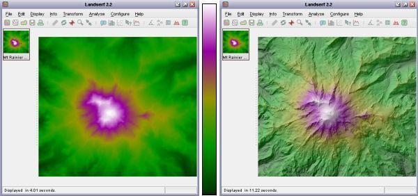 Raster and shaded relief display with default colour table
Various settings for the shaded relief calculation may be set from the configure->Shaded relief...
menu option or the ![]() button. Each
of the parameters can be changed in realtime by moving the relevant slider. The small thumbnail image shows
the effect of these changing parameters on the surface.
button. Each
of the parameters can be changed in realtime by moving the relevant slider. The small thumbnail image shows
the effect of these changing parameters on the surface.
The position of the 'sun' illuminating the surface is controlled by the azimuth and elevation
sliders. Lower sun angles give more pronounced shadowing effects, while azimuths from a southerly or
easterly direction give the impression of inverted topography. The relative balance of the colour and
shading can be controlled using the Percent shading slider. Vertical exaggeration can be used
to control the degree of shadow throughout the whole image and is particularly useful for larger DEMs representing non-mountainous
terrain. The Aspect bias slider controls the degree to which slope direction (aspect) rather than
slope steepness controls the amount of shadow. Higher values will tend to emphasise local detail in the surface and is
particularly useful for detecting error artifacts in elevation models. Lower values will tend to produce more realistic shading.
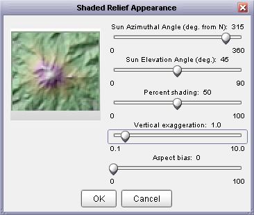 Shaded relief parameters
After pressing OK in this window, the main raster display will be updated with the new settings.
Vector maps are displayed by selecting the Display->Vector menu. This menu item is
toggled on and off with further selection. Colours are assigned to vector values using interpolation of
colour rules in an identical way to rasters.
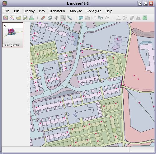 Vector map with points, lines and polygons
The appearance of vector maps can be controlled through the editing of its colour table (see below)
and by altering their appearance using the Display->Vector appearance menu item. This
brings up a window as shown in the figure below that allows the width of vector points and lines to be
set, as well as the transparency associated with vector polygons. Transparent polygons allow multiple
features to be shown overlapping the same area on the ground. Polygon boundaries can be turned on or off,
and their colour can be set by clicking on the small square representing the current boundary colour.
Labels associated with point objects in the vector map can be optionally displayed by ticking the
Show labels box. The appearance of these labels can be controlled by selecting an appropriate
foreground and background colour (click the coloured square to change it). Particularly useful is the ability
to change the transparency of the background. By using semi-transparent background colour, sufficient contrast
with the foreground lettering can be used without obscuring any underlying map data (see figure below). The size
of the labels can controlled with the slider. When displaying labels is often useful to select an appropriate
textual attribute from the attribute table (see Section 3.3).
The vector appearance dialogue can also be used to set higher quality rendering of vector objects
(Optimize for quality), or faster rendering (Optimize for speed).
 Vector display properties and sample output
Any vector or raster map can be enlarged by placing LandSerf into zoom mode. This is achieved either
by selecting the Display->Zoom mode menu option or by toggling the
![]() button. When in zoom mode, dragging
the mouse up and down over the main display area with the left mouse button pressed will zoom in and out
of the displayed image. Dragging the mouse with the right button pressed (or <shift> left button) will
allow a zoomed image to be panned in any direction. To reset a view back to its full extent select either the
button. When in zoom mode, dragging
the mouse up and down over the main display area with the left mouse button pressed will zoom in and out
of the displayed image. Dragging the mouse with the right button pressed (or <shift> left button) will
allow a zoomed image to be panned in any direction. To reset a view back to its full extent select either the
Display->Full image menu option or the ![]() button.
button.
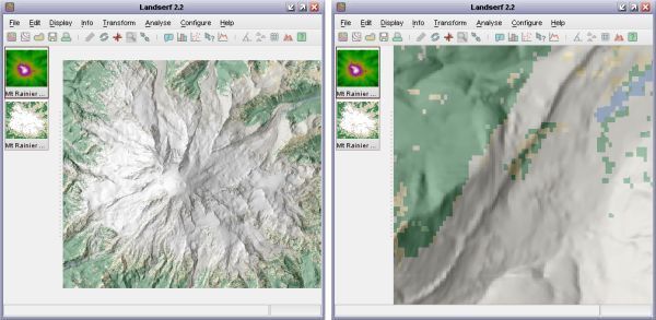 Surface with full extent (left) and zoomed-in area (right)
In order to visualise two surfaces simultaneously, it is possible either to blend the Red, Green, Blue
values together, or to blend the hues of one surface with the saturation of the other. Both are selected
from the Display menu.
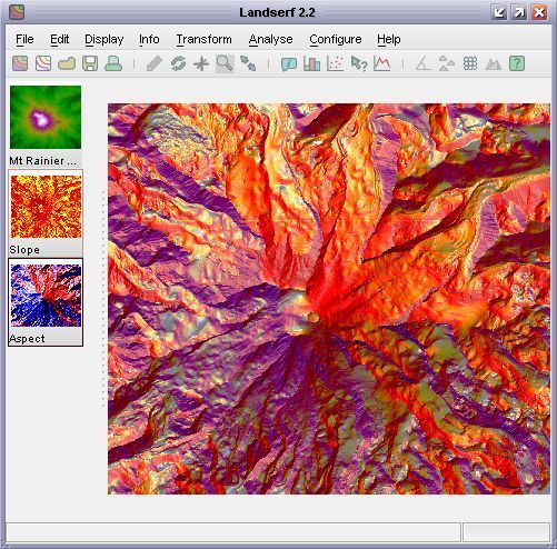 RGB blended slope and aspect map
When choosing the blend option, the percentage weighting given to the primary raster is
required. The closer to 100%, the closer the blended image will resemble the colours of the primary
raster.
Alternatively, the primary and secondary rasters can be mixed by combining the saturation (the 'greyness') of the primary raster and the hues of the secondary raster. Such combination can be particularly useful for representing uncertainty, with stronger saturation indicating greater certainty.
The colour tables associated with either vector or raster maps may be modified by selecting
Edit->Edit Vector or Edit->Edit Raster and then clicking the Edit
button adjacent to the displayed colour bar. Colour tables are defined by a series of colour rules
that associated one or more attribute values with one or more colours. Discrete colour rules link
a single attribute with its own colour while continuous colour rules are used to interpolate a range
of attributes with a range of colours. Both discrete and continuous colour rules can be defined either
graphically or numerically (see Figure below).
 Graphical (left) and numerical (right) colour editor
The colour editor window will allow you to select one of several preset colour tables useful for mapping
onto continuous attributes such as elevation. The colour table is selected by choosing an appropriate colour
scheme from the drop-down menu towards the bottom of the colour editor window. Once defined, colour rules
can be modified by dragging the small vertical tic marks below the colour bar. These increase or decrease
the attribute values associated with a given colour rule. A single colour can be changed graphically by
double-clicking on one of the tic marks to bring up a colour chooser (see figure below).
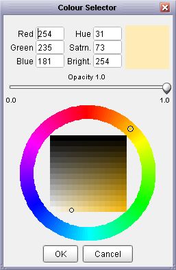 Graphical colour selector
For greater precision, colours tables can be edited numerically by selecting the Numeric
tab at the top of the colour editor window. Each rule is defined by 5 numbers. The first is the attribute
associated with a given colour. The remaining 4 numbers represent the red, green, blue
and alpha (transparency) components of the colour. For continuous colour rules, LandSerf will interpolate
between these colours to produce a continuous colour range.
Colour tables may be saved for later use or shared use between spatial objects. This can be particularly
useful for frequently used datasets such as landcover maps that use particular IDs to represent particular
categories of information. The data sub-directory of LandSerf contains an example colour table
file for representing USGS landcover maps (see the tutorial for an example of
its use).