
Tracing the geometric skeleton of the vasculature of a tumour
The analysis of the vasculature of a tumour can be based on the some of the geometric parameters of the vessels, such as diameter of the vessels, number of branching points, length between branching points, or density of vessels in a given area. The following example illustrates how to perform the geometric analysis using MATLAB and some specifically designed funcions. The analysis is based on a technique called "Scale Space" which progressively blurs an image to observe its characteristics at different "scales": fine details will be observed at the first scales and then will be erased as the image is filtered, whilst larger characteristics will dominate the lower scales. For more detail, the paper by Lindeberg explains the technique: (http://www.nada.kth.se/~tony/earlyvision.html)
Contents
Reading the images
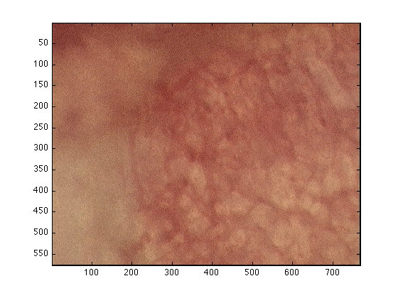
First, the images to be analysed have to be read into MATLAB. If the file is in the working directory one way of reading the data is with 'imread' and 'imagesc' can be used to display it as a figure:
dataIn= imread('wt_010906_mouse7_60minsROI2.bmp');
figure(1)
imagesc(dataIn)
Drag and Drop
Another easy way of importing data into matlab is to drag-and-drop a file from the Finder into the command window of MATLAB, an import wizard window is opened and you normally only need to click on finish before the data is imported into MATLAB. Be aware that in this case, the data will be imported with its particular name, such as 'wt_0101...'. A line similar to this one will appear in the command window of MATLAB:
uiopen('/Users/vasculatureJune2009_10/wt_010906_mouse7_60minsROI2.bmp',1)
To make things easier for future analysis, it is convenient to assing the data to the variable 'dataIn':
dataIn=wt_010906_mouse7_60minsROI2;
Obtaining the skeleton and parameters
Once the image has been read, the function 'scaleSpaceLowMem' will be used to trace the vasculature. In this process, several parameters will be automatically calculated such as diameter of the vessels, length, average length,... The function receives as input the image (that is the variable 'dataIn'), the scale (for images with rather thin vessels use 1:10, if it has thicker vessels try 1:20 or very thick vessels try 1:35) and a calibration parameter; for images that are 'x2.5' use 7.0 , for 'x10' use 1.75 and for 'x20' use 0.88
[fRidges,fStats,netP,dataOut,dataOut2,dataOut3,dataOut4] = scaleSpaceLowMem(dataIn,1:10,1.75);
          Generate Scale Space
          Calculate derivatives in the gradient direction
          Generate Ridge Surfaces
          Calculate Ridge Strength
          Calculate Ridge Saliency
          Calculate Final Metrics
Output of the function
The function returns 7 variables:
fRidges : Final Ridges, a 3D matrix of all ridges obtained at its correct scale
 fStats        : Final Statistics a [N x 5] matrix that contains the individual parameters for each of
                 N ridges traced.
 netP          : Network Parameters many parameters among which the following are available
 netP.numVessels                 number of vessels
 netP.totLength                  total length of the vessels
 netP.avDiameter                 average diameter of all the vessels
 netP.avLength                   average length of the vessels
 netP.totLength_top10            total length of the 10 most important vessels
 netP.avDiameter_top10           average diameter of the 10 most important vessels
 netP.avLength_top10             average length of the the 10 most important vessels
 netP.numLongVessels             number of vessels with longer than 20 pixels
 netP.totLengthPerArea_um2       total length of the vessels per square micrometer of area
 netP.relAreaCovered             ratio of the pixels covered by the all vessels over the total image
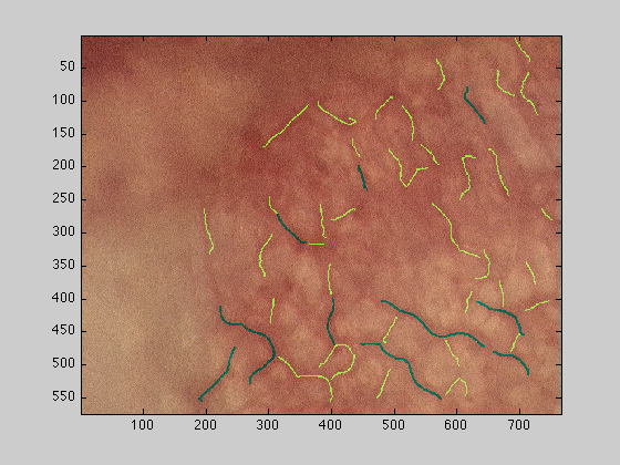
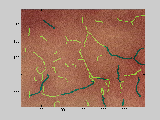
Top 50 vessels
dataOut : The original image with the top 50 vessels overlaid, top 10 in green, 11-50 in yellow
figure(2);imagesc(dataOut);
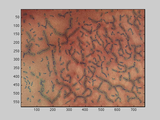
All vessels
dataOut2 : The original image with all vessels overlaid, top 50 as above and the rest in black
figure(3);imagesc(dataOut2);

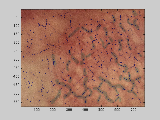
Mask and vessels
dataOut3 : The original image mask of the vessels relative to their width in grey
figure(4);imagesc(dataOut3);
Mask of the top 50
dataOut4 : The original image mask of the top 50 vessels relative to their width in grey
figure(5);imagesc(dataOut4);
Cropping the input data
To select a subsection of the image to analyse, the first way is to pass the variable with the corresponding rows and columns subset, for instance if the original image has dimensions [576 x 768 x 3], and we need to process just the upper left hand region, we can do this by passing 300 rows and 300 columns to the function:
[fRidges,fStats,netP,dataOut,dataOut2,dataOut3,dataOut4] =  scaleSpaceLowMem(dataIn(1:300,1:300,:),1:10,1.75);
figure(6);imagesc(dataOut);
          Generate Scale Space
          Calculate derivatives in the gradient direction
          Generate Ridge Surfaces
          Calculate Ridge Strength
          Calculate Ridge Saliency
          Calculate Final Metrics
Code
To run this code you will need Matlab, the Image Processing toolbox and the following files:
- BranchPoints
- EndPoints
- calculateDataOut
- calculateRidgeParams
- findVessBoundary
- gaussF
- padData
- removeBranchRidges
- removeImageOutliers
- removeThickRidges
- scaleSpaceLowMem
- zerocross
which are all contained in the following zipped file --> scaleSpace.zip <--.
