Chapter 17 Accessing Python and the basic user interface
17.1 Using Python on City University PCs
There are various ways to access Python. A popular method is to install Anaconda, which is a toolkit which provides access to both Python and R (as well as several other packages used in data science and machine learning). Although this is a commercial product, it is free to download for individual use.
In this module I will assume you are using Spyder as the Python interface, which is one of the packages provided by Anaconda. If you go on to work with R you will find that RStudio (a popular front end for R) is also provided by Anaconda.
On City University machines you can run Anaconda by first starting a virtual machine by using your web browser to go to
Login with your usual City details, and select the Make My Reservation button. (There are only a limited number of places available in the virtual lab so you may find it full at peak times.) This will launch a virtual machine running windows where you can access Anaconda.
If you type Anaconda in the Windows search bar at the bottom of the screen and pick the Anaconda Navigator option that appears, then a window should open with lots of icons for different software packages you now have access to. We will be using Spyder in this module. Alternatively you can type Spyder in the search bar and run this direct.
You may prefer to use Colab via a web brower, as described in Section .
17.2 Using Python on your own machine
To install Anaconda at home just go to
and select Individual Edition from the Products list at the top of the page. Download the version of Anaconda for your operating system and follow the installation instructions. You will only need to do this once and then will have access to Spyder (and other packages) every time you use your machine.
17.3 Alternatives to Spyder for running Python
A common alternative to using Spyder for running Python is Jupyter Notebook. This is also available as an option in the Anaconda start screen. This looks a little different from Spyder, as the code is entered into cells instead of a separate panel, and the output appears below the corresponding cell, but it is easy to find online guides to get you started.
It is even possible to write and run Python code without installing anything on your computer. Google provide a free online service called Google Colab at
https://colab.research.google.com
where you can write code in a similar interface to that used by Jupyter notebooks. There is a helpful Getting Started section which explains how this works and provides some examples. To use this you will need to have a standard Google account.
You may find Colab more convenient when working on a City machine. We will describe the basics of using Colab in Section 17.6.
17.4 The basic Spyder interface
When you open Spyder you will see a version of the interface shown in Figure 17.1. However, when you first do this it may look rather different.
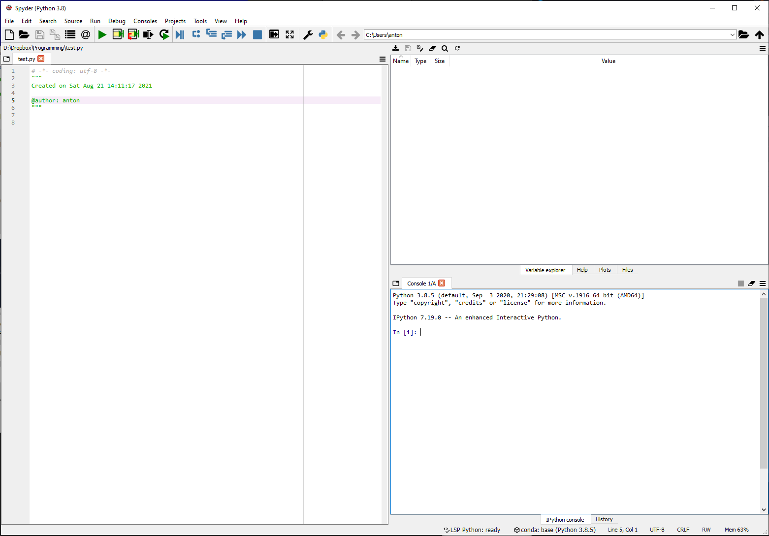
Figure 17.1: The Spyder interface
First, you will probably have a dark version of the interface. I have changed this to a white background partly so that screen grabs will display better in slides and this Handbook, and partly because when we use SymPy later the black background messes up some of the display of mathematics. To change to a white background go to Tools in the top ribbon and choose Preferences. Then choose Appearance on the left and change the Syntax highlighting theme from Spyder Dark to Spyder.
Second, the version of Anaconda on my machine comes with Spyder 4.1.5. By the time you use Spyder this may have been updated to Version 5.2.0 (or later); the icons in the ribbon will look different but for our purposes this will be largely cosmetic.
At first sight this may look quite similar to the VBA window in Excel, but it has some important differences. The large pane on the left is the Editor where we write Python code that we wish to save in a file. The name of this file is displayed at the top of the pane, just below the directory where it has been saved.
Unlike in VBA, there is another pane that we will need to use all of the time. On the lower right we have the iPython Console where we can enter Python code interactively, and where Spyder will display the results of the code that we run from our programs.
Above this pane is a final set of four panes accessed by a series of tabs just above the Console. These include a Help pane, a File Explorer and a Variable Explorer, but importantly also include the Plot pane where any graphical outputs will be displayed. (Spyder 5 also includes Find, Profiler and Code Analysis panes, but we will not use these more advanced features in this module.)
17.5 Entering code into the editor
Unlike in VBA, we now have two different ways to enter code into our editor. We can enter code interactively, a little like we are using a very powerful calculator. To do this we enter each individual line of code into the iPython Console; when we press Return the result of our code is displayed.
A simple example can be seen in Figure 17.2. Each of our inputs is displayed on a line starting with In and the result (if any) is on the following Out line. In the example you can see that as well as basic maths operations we can assign values to variables, which are remembered and can be used in later calculations. We can also print out results in various ways using the print command. Do not worry about the details here; we will explain the basic syntax of Python in the rest of the module.

Figure 17.2: Using the iPython Console
We will rarely using this interactive method for entering code — but the Console window will still be very important as it is where the results of our programs will be displayed and where user input occurs.
The second way of entering code is much more like that used in VBA, where we enter a program into the Editor and then run it after we have finished. Just as in VBA, the Editor is designed to assist us in writing valid code by using highlighting and formatting to help us avoid making mistakes. This will be even more important when we write Python code, as we will see that indentation is no longer optional, as it plays a key role in how our code will be interpreted.
Figure 17.3 is an example of some Python code entered into a file called implicitplot.py. When we save files in Python they have the .py suffix to identify them as Python code. Do not worry about the details of the code — these will all be explained later in the module — but notice how the editor has added colour in various places to highlight certain features of the code.

Figure 17.3: An example of code in the Spyder Editor
Once we have entered the code into the editor, we have to run it. Just as in Excel we can do this by clicking on the Run icon in the top ribbon. When we do this the console window automatically displays a command on an In line as in Figure 17.4 followed by the output (if any). We could have entered this command to run our code, but it is much easier just to press the Run button.

Figure 17.4: Output from our code example
In this case the code generates a graph of a circle; by default this will not appear in the Console, but instead in the Plot pane above, but in this example I changed the settings of the Plot pane (by clicking on the three lines in the top right corner) and unchecked the Mute inline plotting option. This means that any plots are displayed in the console as well as in the plot window.
17.6 Using Colab
Google Colaboratory (usually referred to just as Colab) is a free service (at least in the basic version) provided by Google which can be used to write and run Python code through your web browser. To access this you will need to create a Google account (for example gmail) as the files that you create will be stored in your Google Drive.
The first time you open
https://colab.research.google.com
you should see something like the page shown in Figure 17.5. The main column of text is both an introduction to Colab and an example of a typical file. Colab files (like Jupyter files) are called notebooks and saved as .ipynb files. The reason they are different from ordinary Python files is that they allow you to write both code and text in the same file in separate blocks.
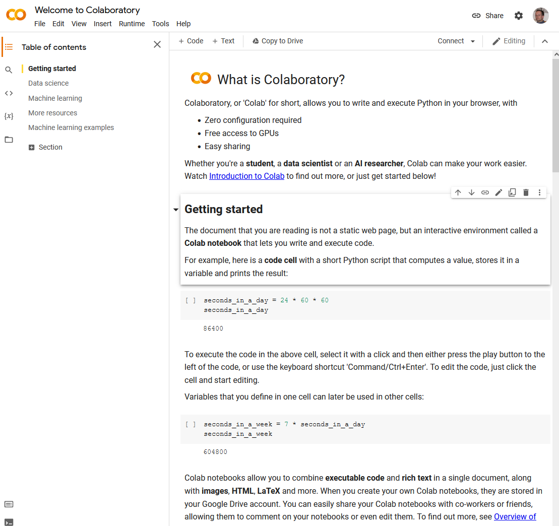
Figure 17.5: The initial view of Google Colab
In the example you see that the file starts with some formatted text, and then had a grey box with some code in it (starting seconds_in_a_day). At the start of each code box is a pair of square brackets; when you put your mouse over these a play icon appears. Pressing this icon runs the code in the given code box. The output is displayed immediately below the box of code. This means that you can have different sections of code in different code boxes, and run each section separately.
At the top of the Figure you can see the menu bar. The file name is the title at the very top, which can be edited. The File option allows you to create new notebooks, or open or save existing ones, and the other menus provide additional features which are best understood by experimenting.
In the righthand top corner there is a dropdown menu labelled Connect. If you ignore this and run your code it will automatically look for a virtual machine in the cloud to run your code on. This can take a few seconds, and so running code through Colab is not as fast as using Spyder and running code on your own machine. There are also restrictions on the resources available to you (but these are very unlikely to matter for the kind of work we are doing in this module).
This Google start file contains lots of examples as well as useful links to further guides, and is a very good place to start to learn how Colab works.
17.7 Help and error detection
Spyder and Colab provide a number of tools to help the user write valid code. As well as automatically indenting where appropriate, they will also provide auto-complete suggestions for Python commands. Hovering over an object in the editor will usually provide a pop-up which describes the object in question; clicking on this pop-up (in Spyder) provides further help in the Help pane above the Console.
Despite all of the above aids, it is inevitable that you will make errors. When Python detects an error it stops running the program and prints an error message in the Console window. This will provide an indication of where the error occured, and what caused it, and can be a very useful tool for debugging your code. For example, consider the code in Figure 17.6.
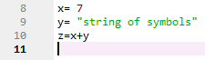
Figure 17.6: An example of some faulty code
This code attempts to add a number and a string, which is not allowed. When the code is run Python provides an error message as in Figure 17.7. Here you can see that after the code is run the traceback identifies the file and line where the error occurs, and gives a message describing the type of error that it has identified. When you have problems with your code these error messages can be very helpful.

Figure 17.7: A traceback of an error in our faulty code