Chapter 23 Working with arrays using NumP
23.1 Arrays
An array in NumPy has to contain elements of the same type. In NumPy the standard numerical types int, float, and complex have extra refinements and you may see types such as int64. These allow for different levels of precision (rather like the different between Int and Long in VBA). However, we can ignore these subtleties and continue to use the standard three types.
We have seen a number of ways of creating a NumPy array in lectures. These included entering the entries one by one, creating an array of the desired shape and filling it with repeated entries, creating an identity matrix, and two special one-dimensional arrays called arange and inspace. Here are some other methods that may sometimes be useful. In what follows, remember that we could also use the optional dtype argument to set the type of the array elements.
First, we shall mimic the method of list comprehension to construct an array. This is best illustrated with an example: the command
np.array([range(i, i+3) for i in [2,4,6]])
produces the 2-dimensional array shown in Figure 23.1.

Figure 23.1: Creating an array with comprehension
Notice that the print command formats the output of a (2-dimensional) array quite nicely, removing the commas between list items and presenting each row on a new line. If we use the console interactively the output is not quite so nice, but still very readable. For higher dimensional arrays the output is a little more complicated (but still much more readable than for the corresponded collection of nested lists in standard Python!).
We can also create an array with a random collection of elements. This is useful if we want to run some simulations of random events. If we consider the arrays
dd = np.random.random((3,3))
ee = np.random.normal(0, 1, (2,2))
ff = np.random.randint(0, 5, (2,2))
then
ddis a 3x3 array of uniformally distributed random variables between 0 and 1.eeis a 2x2 array of normally distributed random variables with mean 0 and standard deviation 1.ffis a 2x2 array of random integers between 0 and 4 inclusive. (Note that as with a slice, the upper bound of 5 is not itself allowed.)
It is also possible to create a new array from another by changing the shape of the array. This can get quite complicated (and does not always do what you might naively expect) so we will only consider here the case where we want to convert an array with one row to an array with one column.
If we know the size of our array then this is very easy. For example, if we have an array x containing a single row with 10 elements then we can create the corresponding column array y with
y = x.reshape(10,1)
This relies on knowing the number of elements in our initial array, which you may not know (for example, if the array has been imported from some real-world data). If you need to know the dimensions of an array then the shape method is useful. For example, if x is the array in Figure 23.1 then x.shape is the tuple (3,3), indicating there are three rows and three columns.
Alternatively, you could convert a one dimensional array x into a two dimensional array y
with one column using the command
y = x[:, np.newaxis]
Here we are using a slice to copy all of the elements of x, and indicating that a new second coordinate is being added with the function np.newaxis. The order is important: if we swapped the colon and the np.newaxis in the expression then we would get a two dimensional array containing one row instead! This is different from what we start with as we now use two coordinates to reference the entries instead of one. The advantage of this method is that we did not need to know the size of x.
There is a transpose function which takes an array of shape (a, b) to an array of shape (b, a). However, this does not immediately replace the above methods as it requires a two-dimensional array before it has any effect. Given a two dimensional array x the transpose is given by x.T (where for once we use a capital letter!).
Finally, we can also create a new array from a pair of two-dimensional arrays (with either the same number of rows or the same number of columns) by stacking the arrays vertically or horizontally. For example if we print out the final_a and final_b arrays
top = np.array([1,2,3,4])
bottom = np.array([5,6,7,8])
final_a = np.vstack([top, bottom])
final_b = np.hstack([top. bottom])
then we get the results shown in Figure @ref(fig:stackout}).
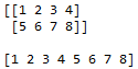
Figure 23.2: The result of stacking arrays vertically and horizontally
23.2 Functions on arrays
There are many functions provided by NumPy that can be used on arrays. Some of these were mentioned in lectures; here is a slightly longer list but there are still many more. All of the standard mathematical functions are available: given an array x we have
| \(\ \) | \(\ \) | \(\ \) |
|---|---|---|
np.sin(x) |
np.cos(x) |
np.tan(x) |
np.arcsin(x) |
np.arccos(x) |
np.arctan(x) |
np.exp(x) |
np.power(n,x) |
np.abs(x) |
np.log(x) |
np.log2(x) |
np.log10(x) |
Most of these are self-explanatory. The function np.power(n,x) corresponds to raising n to the power of x, so if x = np.array([1, 2, 3]) then np.power(3, x) is the array with entries 1, 9, and 27. The functions np.log2 and np.log10 give logs to base 2 and 10 respectively.
All of the standard arithmetical operators +, -, *, /, **, //, % can be used to combine two arrays of the same shape, and in each case the corresponding arithmetic operation will be carried out on the corresponding element in each array. So, for example,
np.array([1, 2, 3]) + np.array([4, 5, 6])
will give array([5, 7, 9]).
As mentioned in lectures, we need to remember that the produce of two arrays given by the multiplication symbol does not correspond to matrix multiplication, for which the @ symbol is used instead.
In lectures we also briefly touched upon the notion of broadcasting, where we try to combine arrays of different dimensions using an arithmetic operation (or some other binary function). As mentioned there, this is rather complicated in general; rather than explain the general case here we will give a few examples to illustrate the special cases introduced in lectures.
Let us suppose that x and y and z are respectively the arrays
Then x + 2, x + y, and x + z are respectively
Here we have added nine copies of the number 2, and three copies of each of y and z, to x.
Given an array x containing numbers we can calculate the following statistical functions for the entire collection of elements of x:
| \(\ \) | \(\ \) | \(\ \) |
|---|---|---|
np.max(x) |
np.min(x) |
np.sum(x) |
np.mean(x) |
np.std(x) |
np.var(x) |
np.median(x) |
np.percentile(x,n) |
np.cumsum(x) |
Again, most of these are obvious. The functions np.std(x) and np.var(x) compute the standard deviation and the variance of the set of entries, and the function np.percentile(x,n)
computes the \(n\)th percentile of x where \(n\) is between 0 and 100.
A slightly less obvious command is np.cumsum(x) which computes the cumulative sum of the array. This returns a new array where the entries are the running totals of the entries in the original array. For example if x = [1, 2, 3, 4, 5] then
np.cumsum(x) = [1, 3, 6, 10, 15].
If we want to compute any of these functions by row then we can add the optional axis=1 to the argument of the function, and for columns add the optional axis=0. So if x is the square array of numbers from 1 to 9 as above, then
np.max(x, axis=1) = [3, 6, 9] \(\quad\quad\) and \(\quad\quad\)
np.max(x, axis=0) = [7, 8, 9]
You may be surprised that the options axis=0 and axis=1 are not the opposite way round. The reason is that this option tells Python which dimension to collapse, but as this is rather confusing it is best to learn (or look up) the relevant command.
23.3 Comparisons and masks
The basic masking methods were covered in lectures. Here we will introduce another useful pair of commands, and then conclude with an example illustrating why NumPy is not always the right tool for the job.
The np.any and np.all commands can be use to determine whether any or all of the values in array satisfy the given condition. For example
np.any(x<0)
will be True if there is at least one negative value in x and False otherwise. Just as for np.sum etc., we can add the optional axis parameter to consider each row or column separately.
We will illustrate this with a slight more complicated example than those we have seen in class. This will also illustrate some of the limitations of using NumPy, which will motivate our study of the Pandas module.
Suppose that we have a group of 4 students who are each taking 5 different modules. We will assume that we are given their marks in an array called marks where each row corresponds to a different student. We wish to calculate their final result.
Let us suppose that the following rules apply. First, a student who fails to get at least 40 in every module will have to resit. If a student does not have to resit then they will get a first if their average is at least 70, a 2:1 if their average is at least 60 but less than 70, and so on.
Here is some code which could solve this problem.
import numpy as np

marks = np.array([[13, 51, 65, 42, 38],
                  [49, 52, 81, 78, 79],
                  [75, 80, 85, 90, 70],
                  [45, 52, 58, 49, 60]])

passed = np.all(marks>=40, axis=1)
average = np.mean(marks, axis=1)
result = np.full(4, "x", dtype="U5")

for i in range(4):
    if passed[i]:
        if average[i] >= 70:
            result[i] = "1"
        elif average[i] >= 60:
            result[i] = "2-1"
        elif average[i] >= 50:
            result[i] = "2-2"
        else:
            result[i] = "3"
    else:
        result[i] = "Resit"

print(result)
We begin with an array of marks, and we can see that the first student has failed (with a 13 in the first module) but the rest have passed.
It is easy to use a mask to determine who has passed, and this gives us the passed array in our example. Similarly, NumPy allows us to easily calculate the average for each student, which we store in the array called average.
Now we would like to store our result in an array of strings. In the code I have set up a dummy array using np.full and putting an “x” in each entry. If we do this and run our code the result will not be correct — we will come back to this shortly.
Next we loop over our result array and check if student i has passed. If they have we determine their result based on their average, and if they have not we set their result to "Resit".
Now if we run this code without the mysterious dtype="U5" then the result is surprising. We get the output in Figure 23.3.

Figure 23.3: The output if the dtype="U5" is omitted
This is because the NumPy array structure is very strict about having all entries of the same type. Not only does it want only integers, or only floats, or only Booleans, but with strings it wants to know their lengths. So the dtype command in our code sets the type of the entries to be strings of up to 5 characters (we chose 5 so that “Resit” would fit), and with that we do get the desired result.
The need for a NumPy array to only contain variables of the same type is one weakness of this solution to our example above. Another is that we have had to work with an array without any identifiers for which students correspond to each row, and which modules correspond to each column. We would more naturally expect to have a set of data where the rows were labelled by student names, and the columns by module names.
This kind of structure is precisely what the Pandas module is designed to deal with.