User Manual for shadingCorrection
The shading correction algorithm is described in detail in:Reyes-Aldasoro, C.C., Retrospective shading correction algorithm based on signal envelope estimation, Electronics Letters (2009), 23 April 2009; Vol. 45, Issue 9, p. 454-456.
Contents
Introduction
A common phenomenon in biomedical imaging is the presence of spurious intensity variations due to the sample of interest and the technique of acquisition. In light microscopy, the variation may originate from uneven sample thickness, out-of-focus objects (in thick slices), or departure from Kohler illumination and is commonly known as shading. In magnetic resonance imaging, intensity inhomogeneity or bias field may be caused by variation in the radio-frequency (RF) coil uniformity, static field inhomogeneity, RF penetration, as well as the anatomy and position of the sample.
This webpage will show you how to use an image-processing algorithm for the retrospective shading correction. The algorithm is fully automatic, the details are described in this paper:
Reyes-Aldasoro, C.C., Retrospective shading correction algorithm based on signal envelope estimation, Electronics Letters (2009), 23 April 2009; Vol. 45, Issue 9, p. 454-456.
Loading the data into Matlab
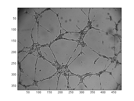
There are two ways to load the data, one is by typing in the command window, for example, to load the image called "image7B.png" you type:
dataIn=imread('image7B.png');
This command would read the tif image and put the values inside the variable called "dataIn". You can change the name of the variable at will. You can also drag and drop, refer to the manual for chromaticity. R*E*M*E*M*B*E*R use only a-z, A-Z, numbers or _ for your file names! myFileName.tif is fine, this%file\of*mine.jpg will create problems in some systems.
To visualise your image you can open a figure and display it like this:
figure(1)
imagesc(dataIn)
Removing the shading
To remove the shading of your image simply type:
[dataOut,errSurface,errSurfaceMin,errSurfaceMax] = shadingCorrection(dataIn);
The Image with the shading removed is stored in "dataOut". To visualise the result type:
figure(2)
imagesc(dataOut/255);
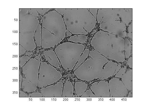
The result (dataOut) is a "double" variable, while the input is a "iunt8" that is why you need the 255 in the end of the imagesc command. Do not worry if you do not understand why, it works fine like that.
To view the effect of the shading and its removal try this:
[rows,columns,levels]  = size(dataIn);

figure(4)
plot([1:columns],dataIn(1,:,1),'r',[1:columns],dataIn(1,:,2),'g',[1:columns],dataIn(1,:,3),'b');
grid on
axis([1 columns 0 255])

figure(5)
plot([1:columns],dataOut(1,:,1),'r',[1:columns],dataOut(1,:,2),'g',[1:columns],dataOut(1,:,3),'b');
grid on
axis([1 columns 0 255])
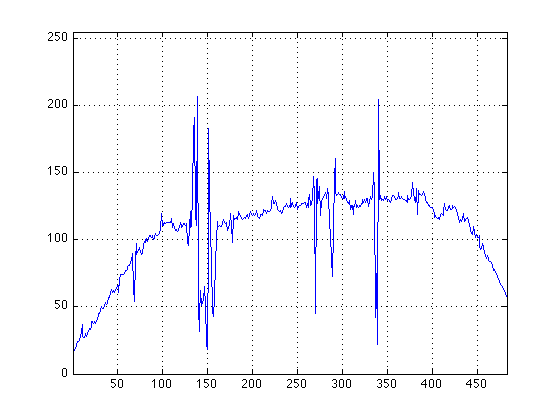
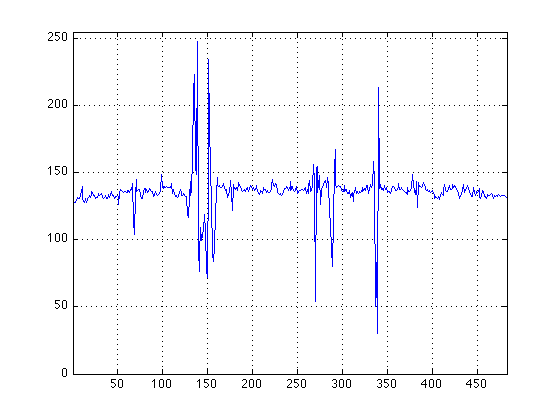
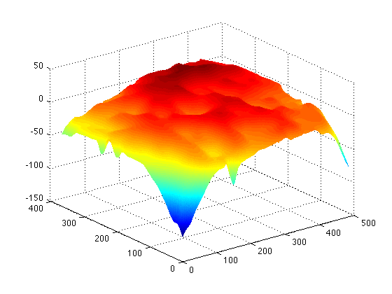
It is evident the difference in shading between both images. To visualise the shading component itself try:
figure(5)

mesh(errSurface(:,:,1))