Chapter 1 The basic Excel interface

Excel, from the Microsoft Office suite of programs, undergoes regular updates which mainly seem to introduce cosmetic changes. Currently a simpler looking interface is favoured, but it is essentially the same as previous versions — just less colourful. The illustrations here may be of older versions of Excel, and so may not be exactly the same visually. But they are similar, and have the same functionality.

On the City University system, you can access Excel from the PCs running Windows 10 by clicking on the Windows icon in the bottom left corner, and then on the green Excel 2019 tile.

Click on the blank workbook icon. Excel is quite a complex set of tools for manipulating data, and the number of options available can seem a little overwhelming at first. We will describe the basic structure of the user interface; many aspects of this will be explained in more detail later in the course.

The most prominent feature (apart from the large blank table) is the ribbon that runs just below the top of the application, as show in Figure 1.1.

Figure 1.1: The Excel ribbon

The top left side of the ribbon lists various high-level menu options (File, Home, Insert, etc.). Clicking on any of these will change the options displayed in the remainder of the ribbon below. These options are also grouped into sections — in the example these are Clipboard, Font, Alignment, etc., and contain the most commonly used commands of each type. At the bottom right of each group there is often a pop-out arrow icon, which will display a more extensive list of commands of the same type. We will discuss how to use some of the many commands available later in the module.

Above the ribbon can be found the quick access toolbar shown in Figure 1.2. This contains the commands that are used so commonly that they should be accessible regardless of the menu item chosen in the ribbon. Initially the only commands available here are (in order) the undo, redo, clipboard and save commands. However, the final icon opens a new menu where further commands can be added to this toolbar. This is a very useful feature, and can even be used to add icons for the new macros that we will write later in the course.

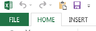
Figure 1.2: The Quick access toolbar

In the middle of the top row is the title of the current file, and a reminder that we are running Excel. When first opened the file has no name, and so is referred to as Book1.

At the far end of the top row are another set of icons, shown in Figure 1.3. These show icons for help, ribbon display options, minimising, maximising, and closing the window. The inbuilt help function is a very useful tool that can answer many of your questions about Excel. If in doubt about how to perform a certain command or operation, this is a very good place to start!

Figure 1.3: The window commands

Just above the main data array can be found the reference area and formula bar, shown in Figure 1.4. The reference area indicates the location of the active cell(s); i.e. the cell(s) currently in use (in this case C3), while the formula bar displays the content of the active cell.

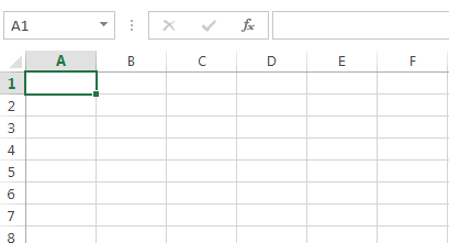
Figure 1.4: The reference area and formula bar

The active cell is marked by a bold frame. If a range of cells is selected (by holding the left mouse button and dragging the cursor) then these will be highlighted with a bold frame, as for the range B2:E5 in Figure 1.5.

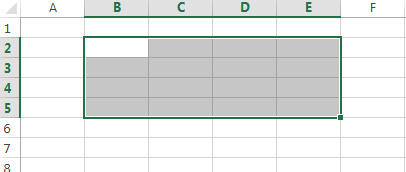
Figure 1.5: The range B2:E5

A single “page” of data is called a worksheet. A single Excel file can consist of many different worksheets, and the collection of such is called a workbook. You can add a new worksheet by clicking on the plus sign. The worksheets in the current workbook are displayed at the bottom of the window, as in Figure 1.6. The active worksheet is the one highlighted — in the Figure this is Sheet 1. To change the active worksheet left-click on the name of the desired sheet.

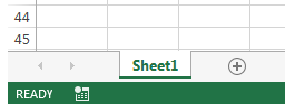
Figure 1.6: Three worksheets, with sheet 1 active

Just as for the workbook itself, the individual worksheets are by default just given numbers, as in the Figure. Worksheets can be renamed, copied, deleted, or reordered by right-clicking on the name.If there are so many sheets that their names do not fit into the space available, then the arrow icons to the left can be used to cycle through them.

In the bottom right corner (shown in Figure 1.7) can be found the scroll bars (for viewing cells which are off the screen). However, it is sometimes more convenient to use the zoom function just below to re-size the whole sheet to enable more data to be displayed. The other icons just to the left of this switch between normal mode and a preview of how the data will appear when printed on the current page size.

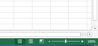
Figure 1.7: The scroll, zoom, and page preview controls