Chapter 3 Built-in Excel functions 1
3.1 Finding functions in Excel
There are many built-in functions in Excel, and initially it can be
hard to work out what functions to use and how. To find functions in
Excel you can go to the Formulas tab and look in
the various categories in the Function Library. Alternatively, if
you can guess roughly how the function might be named, you can start
to type the function name (preceded of course by an = sign) and see
what functions Excel suggests to you. Clicking on one brings up a
brief description of what the function does.
If you have used the Function Library then clicking on a function name
will bring up a box where you can enter the various arguments,
together with a description of the function. For example, if we go to
the Maths functions and click on POWER then the box in
Figure 3.1 appears. We can
either enter the data directly, or
click on the icon at the end of each row, which allows us to choose a
cell (or range of cells) in the worksheet instead. Notice that the
dialogue box also reminds us what kind of data is required in each
argument (in this example two numbers), and will show us the result at
the bottom once we have entered the required data.
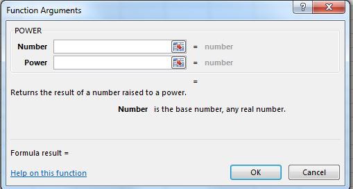
Figure 3.1: The Power function
Once you have found a suitable Excel function, it is usually quicker to
enter it directly rather than via the Formulas
tab. Typing its name and the first parenthesis into a cell will bring
up a reminder of the syntax of the function. Often this is enough to
work out how to use it; if not then the help function (accessible by
pressing the F1 function key) will provide lots of extra information.
3.2 Examples of built-in functions
We cannot hope to describe all of the built-in functions; instead here is a small selection to give an indication of their variety. We will consider a small number of examples from each of the main categories which you are likely to use.
Date and Time Functions
As the name suggests, these deal with properties of dates and times. For example =TODAY() returns today’s date, and =NOW() returns today’s date and the current time.
Financial functions
These deal with a variety of specialised financial functions, which are best learnt in conjunction with a course in finance. We will consider a typical example.
The function =FV gives the future value of an investment. The syntax of this function is
=FV(rate, np, pmt, [pv], [type])
where:
- rate is the interest rate per period
- np is the total number of payments
- pmt is the payment made each period
- pv is the initial lump sum (which if omitted is assumed to be 0)
- type indicates if payments are made at the beginning of each period (1) or at the end (0), and defaults to 0.
For example, suppose you wish to deposit £1,500 into a savings account at a monthly interest rate of 0.27%. You plan to deposit £150 at the beginning of every month for the next 2 years. How much money will be in the account after 2 years?
To calculate this using FV we enter the relevant data, noting that payments and initial lump sums must be entered with a minus sign(!). So the value we want is given by
=FV(0.27%, 24, -150, -1500, 1)
and if you enter this in Excel it will calculate the value to be £5,324.33.
Logical functions
These handle Boolean values, i.e. TRUE or FALSE. We will consider various examples of logical functions in the main lecture notes.
Mathematical and Trigonometric functions
Many of these are standard functions which you would find on a calculator. For example the trig functions
=SIN(x) \(\quad\) =COS(x) \(\quad\) =TAN(x)
where \(x\) is an angle in radians, and the inverse trig functions
=ASIN(x) \(\quad\) =ACOS(x) \(\quad\) =ATAN(x)
The exponential function is =EXP(x), while natural logarithms are given by =LN(x) and logarithms to base 10 by =LOG(x). For logarithms to base \(y\) we use =LOG(x,y). The function =ABS(x) gives the absolute value of \(x\), while =FACT(x) calculates \(x!\). There are many other examples which you can explore in the laboratory sessions.
Statistical functions
These are the functions you will encounter when you study probability and statistics. Examples include =AVERAGE(A1:B7) which returns the arithmetic mean of the values in the range A1:B7, =MAX(A1:B7) which returns the largest value in the range A1:B7, and =VAR(A1:B7) which returns the variance of the values in the range A1:B7.
Text functions
These are functions which manipulate strings of text. Do not forget that when you write text as an argument of a function you always need to use quotation marks!
Examples include =EXACT(text1, text2) which returns TRUE if text1=text2 and FALSE otherwise. This function is case sensitive, so =EXACT(“cat”, “Cat”) has the value FALSE.
The functions =UPPER(text) and =LOWER(text) convert all characters of text to upper (respectively lower) case, while =PROPER(text) converts the text so that the initial letter of every word is upper case and every other letter is lower case.
3.3 Conditional formatting
We have already seen how the format of a cell or range of cells can be changed in various ways. It is often useful to be able to automate this process, so that formatting can be used to highlight key features of the data. This can be done using conditional formatting.
To access conditional formatting go to the Styles
section of the Home tab. First highlight the range of
cells which you wish to format. Clicking on Conditional Formatting
will bring up a series of possible rules, as shown in Figure
3.2, where we show the various Highlight Cells Rules.
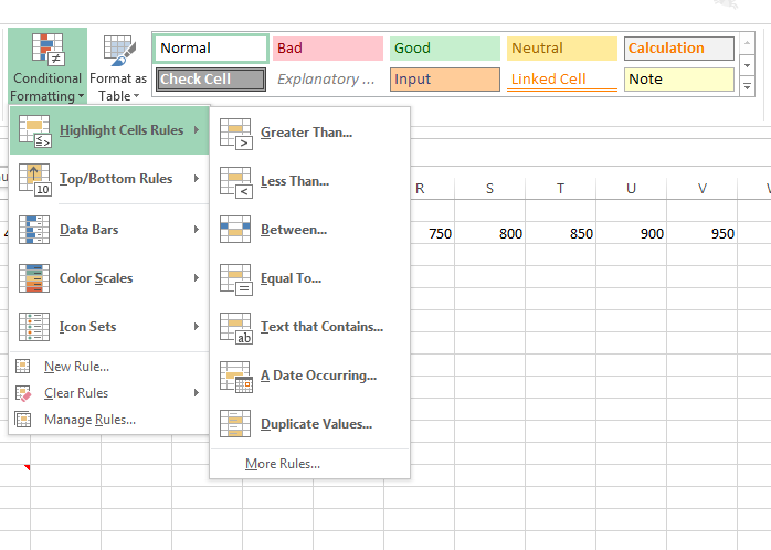
Figure 3.2: The Conditional Formatting options: Highlight cell rules
These and the Top/Bottom Rules, are largely
self-explanatory. The Data Bars option (and the similar
Color Scales option) superimpose either a colour scale
or bars onto the cells. Data Bars can appear in a number of styles, as
shown in Figure 3.3.
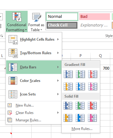
Figure 3.3: The Conditional Formatting options: Data Bars
The Icon Sets use a variety of different kinds of icons
to represent the relative values of the different cells being
formatted. This is based on their values relative to the average of
the given data. The different icons which can be used are illustrated
in Figure 3.4.
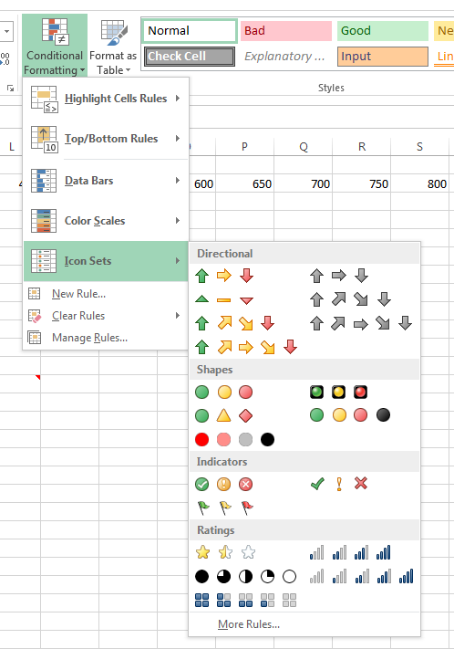
Figure 3.4: The Conditional Formatting options: Icon Sets
Although there are many different kinds of conditional formatting
offered by default, you may wish to construct new rules to highlight
the data in a different way. The New Rule... option in
the Conditional Formatting menu provides many options
for doing this. For example, see Figure 3.5.
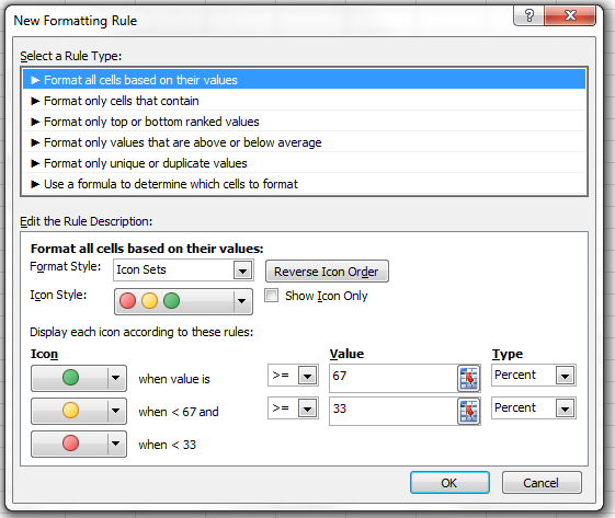
Figure 3.5: The Conditional Formatting options: Advanced Rules 1
To illustrate the various rules in action, consider the data illustrated in Figure 3.6. The first column is formatted using the Highlight Cells rule for all cells with values greater than 10. The same set of data is then given with data bars, and then with the default rules for five colour icons.
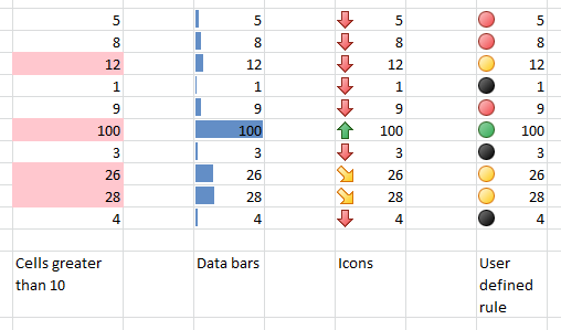
Figure 3.6: An example of conditional formatting
Note that the Icons view is a little unsatisfactory in this case, as the very large value 100 skews the data so that almost all of the other values are in the bottom category. In the final column the same data is given using a custom rule, where the colour of the icons depends on values chosen to suit the given data, as shown in Figure 3.7.
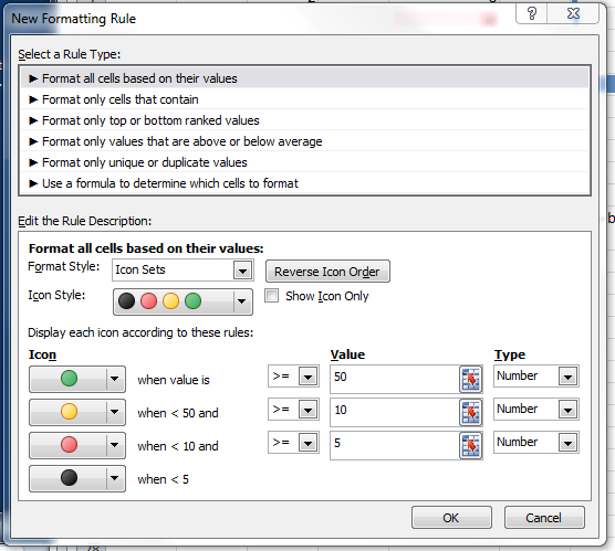
Figure 3.7: The Conditional Formatting options: Advanced Rules 2
If a variety of rules are used in the same worksheet, you can easily
forget which rules apply where, or what they consist of. The
Manage Rules... option in the main Conditional Formatting menu will allow you to display and edit the rules
currently in use.