Chapter 2 Data entry and basic formatting command

When working on a new project, your first action should be to give your workbook a name and save it on your computer. There are several ways of doing this; the easiest is probably to go to the save icon in the quick access toolbar at the top (or the file menu on the ribbon).

When you save the file you will need to give it a name and chose a file type. For now, you will typically chose the option Excel Workbook which saves the document as a .xlsx file. However if you wish to save the file in a format compatible with older versions of Excel, you should probably choose the option Excel 97-2003 Workbook which creates a .xls file.

There are many other options available; later we will need to use the Excel Macro-Enabled Workbook option .xlsm when we work with macros and VBA. You can also choose to publish the document as a pdf, which is useful if you want to send it to people using different operating systems (or without Excel). However, to do this it is best to use the Export option rather than the Save option.

When working on your Excel file, it is good practice to save regularly, either using the save icon or by typing Ctrl+s (i.e. the Control and S keys together). Excel does occasionally crash, and without regular saves you can lose a lot of data.

2.1 Data entry

The easiest way to enter data into a worksheet is to type it directly into the active cell, or into the formula bar. Once data has been entered, the action may be completed in a variety of different ways. Suppose we have just entered data into cell C8. Then

1. Enter moves to the next cell in the same column, i.e. C9.
2. Shift+Enter moves to the previous cell in the same column, i.e. C7.
3. Tab moves to the next cell in the same row, i.e. D8.
4. Shift+Tab moves to the previous cell in the same row, i.e. B8.
5. The cursor keys move in the direction indicated.
6. The tick icon next to the formula bar completes the formula but does not move to a new cell.
7. Esc does not move and cancels all modifications since the last completion of type (1–6) above.
8. The cross icon next to the formula bar has the same effect as Esc, as does the undo icon in the quick access toolbar.

Do not finish the entry in a cell by clicking on another cell as this will produce the wrong result when entering formulas!

If you left-click on a cell you can replace the entry in it; alternatively click on the formula bar if you wish to edit the entry in the active cell. To modify data that has been entered, use Delete or Backspace to delete the data to the right or left respectively of the cursor.

You may have done more than just enter data in a cell; you may also have formatted the cell in a special way, or added a comment (see later). To clear all of these changes use the Home tab on the ribbon, and go to the Editing section at the right-hand end. Here the Clear icon provides a drop-down menu of various types of data which can be deleted from the chosen cell.

To spell-check entries, go to the Review tab on the ribbon, and select Spelling from the Proofing section.

2.2 Formatting data

Once you have entered data into your workbook you may wish to format it, either for aesthetic reasons or to make it easier to work with. The formatting commands can be found under the Home tab in the ribbon, in the Cells section. Clicking on the Format icon brings up a menu of formatting commands, and the final one (Format Cells...) allows you to change various properties of the selected cells, as illustrated in Figure 2.1.

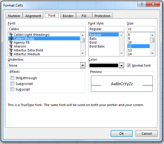
Figure 2.1: The Format Cells option

These properties are grouped into a number of different tabs, called Number, Alignment, Font, Border, Fill, and Protection. Most of these are self-explanatory, and best understood by experimentation. Some of these options can also be accessed directly in the Font, Alignment, and Number sections of the Home tab.

One useful option which can be found in the Alignment tab is the Wrap text option which will help display text which is too large for the cell by splitting it into multiple lines. The Protection tab is very useful, as you can use it to prevent other people from editing certain cells in your workbook, or to hide the content of some of the cells from view.

In certain more complicated tables, or when you want a long title to occupy a number of columns of your sheet, you can merge a range of cells into a single cell. To do this, select the range of cells and then click on the Merge and Center icon in the Alignment section of the Home tab.

It is also possible to add comments to a cell, which do not appear in the cell itself, but instead appear when the mouse hovers over a small mark in the top corner of the cell (as in Figure 2.2. This is done by right-clicking on the cell and choosing the Insert Comment command. To remove such a comment, right-click again on the cell and choose Delete Comment from the menu.

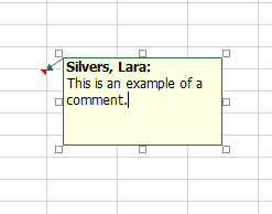
Figure 2.2: Viewing the comment associated with a cell

Often you will wish to have a row or column of data which increases by a constant amount (or by a constant factor) each time. For example, you may wish to fill the column C1-C20 with the numbers 50, 100, 150, …, 1000. There are two ways to do this automatically.

The first is to enter at least two of the starting values (so put 50 in C1 and 100 in C2 for example). Then select the range C1:C2, and move the cursor to the lower right corner of the selection so that the cursor changes from a large white cross to a small black cross. Then drag this corner down to select the desired range, and the entries will be completed for you, when the increase is a linear one.

Alternatively, enter 50 into C1 and use the Fill button from the Editing section of the Home tab. Choosing the Series entry will bring up the box shown in Figure 2.3. Choose the direction to fill (in this example Columns), and the type of fill (in this example Linear). The step value is the amount which each successive entry will be increased by (linear) or multiplied by (growth); this will either fill the range which has been selected or will finish when the value exceeds the Stop value. Thus in our example, we could select C1 and choose a step value of 50 and a stop value of 1000. This option can also be used for a regular series of dates.

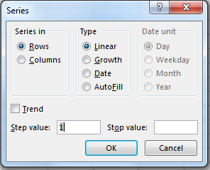
Figure 2.3: Autofilling a series

2.3 Entering formulas

As we have already seen in lectures, formulas in Excel must be preceded by an = sign. If a formula is entered in a cell without this symbol, it will not be evaluated but instead remain as a series of symbols.

When entering a formula that involves references to other cells, one can either enter the cell reference directly, or click on the relevant cell to insert the cell reference. (This will also work for ranges of cells in more complicated functions later on.)

For example, to enter the formula =1/(D5+G4) into the cell B4, one can either enter the formula as just displayed, or instead enter =1/( into B4 followed by clicking on D5, typing +, clicking on G4, and then typing ).

If you enter a formula that does not make sense (for example if you omit the final bracket in the above expression), then Excel will try to guess what you meant and suggest a correction.

To name a cell or range of cells, select them, and in the Formulas tab select the Define Name button. Entering a name in the first dialogue box will enable you to refer to those cell(s) by that name instead of by their cell reference.