Chapter 4 Built-in Excel functions 2
4.1 Information functions and error messages
One of the issues that can cause problems in Excel and VBA (and more
generally is an important issue in any programming language) is when a
function refers to an object that either does not exist or is of the
wrong type. To help the user keep track of the cause of these
problems, Excel includes a variety of error messages. The most common
errors you are likely to encounter are:
- #DIV/0! division by zero
- #NAME? a formula contains an undefined variable or function name, or the function syntax is not valid
- #N/A the value is not available (for example the cell referred to does not contain appropriate data)
- #NUM! a numerical error, for example SQRT(-2)
- #VALUE! an invalid argument type, for example SQRT(text)
- #REF! invalid cell reference
- #NULL! an error of syntax, for example a misplaced space or a comma separating range references
- ###### the entry in the cell is too wide to be displayed
- circular error a formula which refers to its own location
One of the features of a good program is its ability to cope with unexpected errors. Users may enter the wrong kind of input, or unexpected combinations of circumstances may occur. We will see various ways to cope with errors when we look at VBA.
In Excel, Information functions provides information about cell data or format that can be used to avoid or identify errors. Some examples of useful information functions include =TYPE(cell) which returns a number which stands for the type of data contained in the cell referred to:
- 1 number
- 2 text
- 4 logical value
- 16 error value
- 64 array
and =ERROR.TYPE(cell): if the cell referred to contains an error message this returns a number that stands for the type of error:
- 1 #NULL!
- 2 #DIV/0!
- 3 #VALUE!
- 4 #REF
- 5 #NAME!
- 6 #NUM!
- 7 #N/A
and =ISODD(cell) that returns TRUE if the cell contains an odd number and FALSE otherwise.
4.2 Lookup functions
We have already considered VLookup and HLookup functions in lectures. These are very useful but somewhat clunky in their syntax, and with some rather irritating limitations.
Microsoft have recently introduced an improved fuction called XLookup which combines the features of both of these functions and improves their useability considerably. Unfortunately this is only available in certain more recent versions of Excel. For this reason, and because VLookup and HLookup are widely used in existing code that you may encounter in your career, we continue in lectures to consider the older versions of these functions.
However, you may wish to try out the new XLookup command. The format is
=XLOOKUP(value, lookup_array, return_array, [if_not_found], [match], [search])}
Here
- value is the value to search for
- lookup_array is the array in which to look for the value (which can be either a row or a column)
- return_array is the array from which the result is to be returned. This must have the same number of columns (or rows) as the lookup_array or else there will be an error.
- if_not_found is an optional argument which consists of a string in double quotes which will be printed if the value is not found. By default this prints the same error message as VLookup and HLookup: #N/A
- match is an optional argument. By default it looks for an exact match, but there are the following alternatives:
- -1: Exact match. If none found, return the next smaller item.
- 1: Exact match. If none found, return the next larger item.
- 2: Allows for a wildcard match.
- search & is an optional argument. By default it starts searching from the first item in the list, but setting this option to be \(-1\) will result in a search in reverse order from the final item in the list.
There are a number of advantages over the original HLookup and VLookup functions. The value to search for is now exact by default, and the search column (or row) does not not have to be to the left of (or above) the values to be returned.
The function will now also return an array of values; for example if we search down a column for a particular entry, and the return array has multiple columns in it, then the corresponding entries in all of these columns will be returned at the same time. This allows for XLookups to be nested, with both horizontal and vertical searches occurring in the same expression.
As an example, suppose that we have the data shown below in cells B2:E8 of our spreadsheet.
| Name | Height | Weight | Eye colour |
|---|---|---|---|
| Aragorn | 165 | 80 | Blue |
| Theoden | 168 | 83 | Brown |
| Boromir | 177 | 88 | Brown |
| Faramir | 172 | 86 | Blue |
| Elendil | 170 | 90 | Green |
| Grima | 180 | 79 | Blue |
If we enter in cell H4 the command
=XLOOKUP(H3,B3:B8,D3:D8,“Not a valid name”)
then this looks for the content of cell H3 in column B, and returns values from column D. If the value does not exist in Column B it returns the message “Not a valid name”. If cell H3 contains “Grima” then this will return the value 79.
In we enter in cell H7 the command
=XLOOKUP(H6,B3:B8,C3:E8,“Not a valid name”)
then this is very similar, except it now returns three values from columns C, D, and E. If cell H6 contains Aragorn then this will return “165, 80, Blue” in the row of three cells starting from H7.
If we were to enter
=XLOOKUP(87,D3:D8,B3:B8,0,-1)
this would look for 87 in column D and return values from column B. The value 0 means that no message will be returned if the value is missing (which will not be relevant for this example) and -1 means that if there is no exact match then the function will return the next smaller answer. As 87 is not in column D, the next smaller entry is 86, and so the function will return “Faramir”. This example illustrates that there are no problems with inexact searches where the numerical data is not in increasing order, and that we can now return values from a column to the left of the one we are searching in.
4.3 Protecting Worksheets and Workbook
When creating workbooks or worksheets you may wish to protect part or
all of them to make sure that your work will not be changed by
accident (or deliberately). To protect a worksheet or workbook in
Excel you use the Changes section of the Review tab, shown in Figure 4.1.
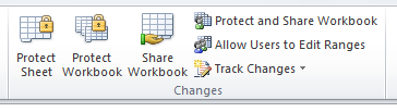
Figure 4.1: The Changes section before protection
Once you have chosen to protect either the worksheet or workbook, you will be able to choose what actions users are allowed to carry out, as shown in Figure 4.2.
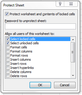
Figure 4.2: Protecting a worksheet
You can also enter a password for added security. Once you have done
this, only users who know the password will be able to unprotect the
sheet again. Once you have done this the Change section
will appear as in Figure 4.3.
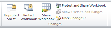
Figure 4.3: The Changes section after protection
You can also use the Changes section to share your
workbook, or to allow users to edit ranges in an otherwise protected
workbook. These and other features are best explored by
experimentation.
You may also want some of the information on the worksheet not to be visible to certain users (it may for example be confidential). To hide cells from view, you must use the formatting commands for cells considered earlier in these notes.